Ansys Coupled Field Analysis 1y4i3y
This document was ed by and they confirmed that they have the permission to share it. If you are author or own the copyright of this book, please report to us by using this report form. Report 3b7i
Overview 3e4r5l
& View Ansys Coupled Field Analysis as PDF for free.
More details w3441
- Words: 69,991
- Pages: 307
5/29/13
Chapter 1. Coupled-Field Analyses
Coupled-Field Guide |
Chapter 1. Coupled-Field Analyses
www.kxcad.net Home > CAE Index > ANSYS Index > Release 11.0 Documentation for ANSYS
A coupled-field analysis is a combination of analyses from different engineering disciplines (physics fields) that interact to solve a global engineering problem, hence, we often refer to a coupled-field analysis as a multiphysics analysis. When the input of one field analysis depends on the results from another analysis, the analyses are coupled. Some analyses can have one-way coupling. For example, in a thermal stress problem, the temperature field introduces thermal strains in the structural field, but the structural strains generally do not affect the temperature distribution. Thus, there is no need to iterate between the two field solutions. More complicated cases involve two-way coupling. A piezoelectric analysis, for example, handles the interaction between the structural and electric fields: it solves for the voltage distribution due to applied displacements, or vice versa. In a fluid-structure interaction problem, the fluid pressure causes the structure to deform, which in turn causes the fluid solution to change. This problem requires iterations between the two physics fields for convergence. The coupling between the fields can be accomplished by either direct or load transfer coupling. Coupling across fields can be complicated because different fields may be solving for different types of analyses during a simulation. For example, in an induction heating problem, a harmonic electromagnetic analysis calculates Joule heating, which is used in a transient thermal analysis to predict a time-dependent temperature solution. The induction heating problem is complicated further by the fact that the material properties in both physics simulations depend highly on temperature. Some of the applications in which coupled-field analysis may be required are pressure vessels (thermal-stress analysis), fluid flow constrictions (fluid-structure analysis), induction heating (magnetic-thermal analysis), ultrasonic transducers (piezoelectric analysis), magnetic forming (magneto-structural analysis), and microelectromechanical systems (MEMS). The following coupled-field analysis topics are available: Types of Coupled-Field Analysis System of Units About GUI Paths and Command Syntax
www.kxcad.net/ansys/ANSYS/ansyshelp/Hlp_G_COU1.html
1/1
5/29/13
1.1. Types of Coupled-Field Analysis
Coupled-Field Guide | Chapter 1. Coupled-Field Analyses |
1.1. Types of Coupled-Field Analysis
www.kxcad.net Home > CAE Index > ANSYS Index > Release 11.0 Documentation for ANSYS
The procedure for a coupled-field analysis depends on which fields are being coupled, but two distinct methods can be identified: load transfer and direct. These methods are described briefly below, and in the following chapters in detail: "Direct Coupled-Field Analysis" Load Transfer Methods "The ANSYS Multi-field (TM) Solver - MFS Single-Code Coupling" "Multi-field Analysis Using Code Coupling" "Load Transfer Coupled Physics Analysis" "Unidirectional Load Transfer" ANSYS also offers the following additional coupled-field methods: "Coupled Physics Circuit Simulation" "Reduced Order Modeling" 1.1.1. Direct Method
The direct method usually involves just one analysis that uses a coupled-field element type containing all necessary degrees of freedom. Coupling is handled by calculating element matrices or element load vectors that contain all necessary . An example of a direct method coupled-field analysis is a piezoelectric analysis using the PLANE223, SOLID226, or SOLID227 elements. Another example is MEMS analysis with the TRANS126 element. A FLOTRAN analysis using the FLOTRAN elements is another direct method. Refer to the Fluids Analysis Guide for detailed procedures for a FLOTRAN analysis. 1.1.2. Load Transfer Methods
The load transfer methods involve two or more analyses, each belonging to a different field. You couple the two fields by applying results from one analysis as loads in another analysis. There are different types of load transfer analyses, explained in the following sections. www.kxcad.net/ansys/ANSYS/ansyshelp/Hlp_G_COU1_2.html
1/6
5/29/13
1.1. Types of Coupled-Field Analysis
1.1.2.1. Load Transfer Coupled Analysis - ANSYS Multi-field solver
The ANSYS Multi-field solver, available for a large class of coupled analysis problems, is an automated tool for solving load transfer coupled field problems. It supersedes the physics file-based procedure and provides a robust, accurate, and easy to use tool for solving load transfer coupled physics problems. Each physics is created as a field with an independent solid model and mesh. Surfaces or volumes are identified for coupled load transfer. A multi-field solver command set configures the problem and defines the solution sequencing. Coupled loads are automatically transferred across dissimilar meshes by the solver. The solver is applicable to static, harmonic, and transient analysis, depending on the physics requirements. Any number of fields may be solved in a sequential (or mixed sequential-simultaneous) manner. Two versions of the ANSYS Multi-field solver, designed for different applications, offer their own benefits and different procedures: MFS - Single code: The basic ANSYS Multi-field solver used if the simulation involves small models with all physics field contained within a single product executable (e.g., ANSYS Multiphysics). The MFS Single code solver uses iterative coupling where each physics is solved sequentially, and each matrix equation is solved separately. The solver iterates between each physics field until loads transferred across the physics interfaces converge. MFX - Multiple code: The enhanced ANSYS Multi-field solver used for simulations with physics fields distributed between more than one product executable (e.g., between ANSYS Multiphysics and ANSYS CFX). The MFX solver can accommodate much larger models than the MFS version. The MFX Multiple code solver uses iterative coupling where each physics is solved either simultaneously or sequentially, and each matrix equation is solved separately. The solver iterates between each physics field until loads transferred across the physics interfaces converge. See "Multi-field Analysis Using Code Coupling" for detailed procedures. 1.1.2.2. Load Transfer Coupled Analysis - Physics File
With a physics file-based load transfer, you must explicitly transfer loads using the physics environment. An example of this type of analysis is a sequential thermal-stress analysis where nodal temperatures from the thermal analysis are applied as "body force" loads in the subsequent stress analysis. The physics analysis is based on a single finite element mesh across physics. You create physics files that define the physics environment; these files configure the database and prepare the single mesh for a given physics simulation. The general process is to read in the first physics file and solve. Then read in the next physics field, specify the loads to be transferred, and solve the second physics. Use the LDREAD command to link the different physics environments and apply the specified results data from the first physics environment as loads for the next environment's solution across a node-node similar mesh interface. You can also use LDREAD to read results from one analysis as loads in a subsequent analysis, without the use of physics files. See "Load Transfer Coupled Physics Analysis" for detailed procedures. 1.1.2.3. Load Transfer Coupled Analysis - Unidirectional Load Transfer
You can also couple a fluid-solid interaction analysis by unidirectional load transfer. This method requires that you know that the fluid analysis results do not affect the solid loads significantly, or vice-versa. Loads from an www.kxcad.net/ansys/ANSYS/ansyshelp/Hlp_G_COU1_2.html
2/6
5/29/13
1.1. Types of Coupled-Field Analysis
ANSYS Multiphysics analysis can be unidirectionally transferred to a CFX fluid analysis, or loads from a CFX fluid analysis can be transferred to an ANSYS Multiphysics analysis. The load transfer occurs external to the analyses. See "Unidirectional Load Transfer" for detailed procedures on both ANSYS-to-CFX and CFX-toANSYS unidirectional methods. 1.1.3. When to Use Direct vs. Load Transfer
Direct coupling is advantageous when the coupled-field interaction involves strongly-coupled physics or is highly nonlinear and is best solved in a single solution using a coupled formulation. Examples of direct coupling include piezoelectric analysis, conjugate heat transfer with fluid flow, and circuit-electromagnetic analysis. Elements are specifically formulated to solve these coupled-field interactions directly. For coupling situations which do not exhibit a high degree of nonlinear interaction, the load transfer method is more efficient and flexible because you can perform the two analyses independently of each other. Coupling may be recursive, where iterations between the different physics are performed until the desired level of convergence is achieved. In a load transfer thermal-stress analysis, for example, you can perform a nonlinear transient thermal analysis followed by a linear static stress analysis. You can then use nodal temperatures from any load step or time-point in the thermal analysis as loads for the stress analysis. In a load transfer coupling analysis, you can perform a nonlinear transient fluid-solid interaction analysis, using the FLOTRAN fluid elements and ANSYS structural, thermal or coupled field elements. Direct coupling typically requires less -intervention because the coupled-field elements handle the load transfer. Some analyses must be done using direct coupling (such as piezoelectric analyses). The load transfer method requires that you define more details and manually specify the loads to be transferred, but offers more flexibility in that you can transfer loads between dissimilar meshes and between different analyses. The following tables provides some general guidelines on using each method. Table 1.1 Choosing a Method Method
Application
Load-Transfer Thermal-structural
Varied
Electromagnetic-thermal, electromagnetic-thermalstructural
Induction heating, RF heating, Peltier coolers
Electrostatic-structural, electrostatic-structural-fluidic
MEMS
Magnetic-structural
Solenoids, electromagnetic machines
FSI, CFX- and FLOTRAN-based
Aerospace, automative fuel, hydraulic systems, MEMS fluid damping, drug delivery pumps, heart valves
Electromagnetic-solid-fluid
Fluid handling systems, EFI, hydraulic systems
Thermal-CFD
Electronics cooling
Direct Thermal-structural
Varied, such as gas turbines, MEMS resonators
Acoustic-structural
Acoustics, sonar, SAW
Piezoelectric
Microphones, sensors, actuators, transducers, resonators
Electroelastic
MEMS
www.kxcad.net/ansys/ANSYS/ansyshelp/Hlp_G_COU1_2.html
3/6
5/29/13
1.1. Types of Coupled-Field Analysis
Piezoresistive
Pressure sensors, strain gauges, accelerometers
Thermal-electric
Temperature sensors, thermal management, Peltiere cooler, thermoelectric generators
Electrostatic-structural
MEMS
Circuit coupled electromagnetics
Motors, MEMS
Electro-thermal-structural-magnetic
IC, PCB electro-thermal stress, MEMS actuators
Fluid-thermal
Piping networks, manifolds
Table 1.2 Methods Available Coupled Physics
Load Transfer
Direct
Comments
Thermal-structural
ANSYS Multifield solver
PLANE13, SOLID5, SOLID98, PLANE223, SOLID226, SOLID227. See StructuralThermal Analysis.
Can also use LDREAD, but we recommend using the ANSYS Multi-field solver if using the load transfer method.
Thermal-electric
ANSYS Multifield solver
PLANE223, SOLID226, SOLID227 (Joule, Seebeck, Peltier, Thompson). See Thermal-Electric Analysis for a complete list of elements.
Can also use LDREAD, but we recommend using the ANSYS Multi-field solver if using the load transfer method.
Thermal-electric- structural
ANSYS Multifield solver
PLANE223, SOLID226, SOLID227 . See StructuralThermal-Electric Analyses for a complete list of elements.
Can also use LDREAD, but we recommend using the ANSYS Multi-field solver if using the load transfer method. Joule heating is ed by both the direct and load-transfer methods. Seebeck, Peltier, and Thompson effects are available only with the direct method.
Piezoelectric
---
PLANE13, SOLID5, SOLID98, PLANE223, SOLID226, SOLID227. See Piezoelectric Analysis.
Electroelastic
---
PLANE223, SOLID226, SOLID227. See Electroelastic Analysis.
Piezoresistive
---
PLANE223, SOLID226, SOLID227. See Piezoresistive Analysis.
Electromagnetic-thermal
ANSYS Multifield solver
PLANE13, SOLID5, SOLID98
Can also use LDREAD, but we recommend using the ANSYS Multi-field solver if using the load transfer method.
Electromagnetic-thermalstructural
ANSYS Multifield solver
PLANE13, SOLID5, SOLID98
Can also use LDREAD, but we recommend using the ANSYS Multi-field solver if using the load transfer method.
Acoustic-Structural (Inviscid FSI)
---
FLUID29, FLUID30
Circuit-coupled
---
CIRCU124 + PLANE53,
www.kxcad.net/ansys/ANSYS/ansyshelp/Hlp_G_COU1_2.html
4/6
5/29/13
1.1. Types of Coupled-Field Analysis
electromagnetic
SHELL99, or SOLID117. CIRCU94. See "Coupled Physics Circuit Simulation".
Electrostatic-structural
ANSYS Multifield solver
TRANS109, TRANS126. See Electromechanical Analysis.
Can also use LDREAD, but we recommend using the ANSYS Multi-field solver if using the load transfer method.
Electromagnetic-structuralfluidic (FLOTRAN-based)
ANSYS Multifield solver
---
Can also use LDREAD, but we recommend using the ANSYS Multi-field solver if using the load transfer method.
Magnetic-structural
ANSYS Multifield solver
PLANE13, SOLID62, SOLID5, SOLID98. See MagnetoStructural Analysis.
Can also use LDREAD, but we recommend using the ANSYS Multi-field solver if using the load transfer method.
Fluid-thermal (FLOTRAN based)
ANSYS MultiFLOTRAN Conjugate heat field solver MFS transfer
Fluid-thermal (CFX - based)
ANSYS MultiCFX Conjugate heat transfer field solver MFX
FSI (FLOTRAN - based)
ANSYS Multi--field solver MFS
FSI (CFX - based)
ANSYS Multi--field solver MFX, Unidirectional ANSYS to CFX Load Transfer (EXPROFILE), Unidirectional CFX to ANSYS Load Transfer (MFIMPORT)
Magnetic-fluid
ANSYS Multifield solver
---
Use the MFX solver if you need to iterate between the separate codes. Otherwise, use the appropriate unidirectional option.
Can also use LDREAD, but we recommend using the ANSYS Multi-field solver if using the load transfer method. LDREAD can read Lorentz forces into CFD mesh. LDREAD can also for conventional velocity effect (PLANE53, SOLID97, SOLID117) by importing CFD calculated velocity distribution to an electromagnetic model to simulate electric power generation.
1.1.4. Additional Analysis Methods
In addition to the methods discussed above, ANSYS also offers the following methods: 1.1.4.1. Reduced Order Modeling
www.kxcad.net/ansys/ANSYS/ansyshelp/Hlp_G_COU1_2.html
5/6
5/29/13
1.1. Types of Coupled-Field Analysis
Reduced Order Modeling describes a solution method for efficiently solving coupled-field problems involving flexible structures. The reduced order modeling (ROM) method is based on a modal representation of the structural response. The deformed structural domain is described by a factored sum of the mode shapes (eigenvectors). The resulting ROM is essentially an analytical expression for the response of a system to any arbitrary excitation. This methodology has been implemented for coupled electrostatic-structural analysis and is applicable to micro-electromechanical systems (MEMS). See "Reduced Order Modeling" for detailed procedures. 1.1.4.2. Coupled Physics Circuit Simulation
You can often perform coupled physics simulations using a circuit analogy. Components such as "lumped" resistors, sources, capacitors, and inductors can represent electrical devices. Equivalent inductances and resistances can represent magnetic devices, and springs, masses, and dampers can represent mechanical devices. ANSYS offers a set of tools to perform coupled simulations through circuits. A Circuit Builder is available to conveniently create circuit elements for electrical, magnetic, piezoelectric, and mechanical devices. The ANSYS circuit capability allows you to combine both lumped elements, where appropriate, with a "distributed" finite element model in regions where characterization requires a full finite element solution. A common degree-offreedom set allows the combination of lumped and distributed models. See "Coupled Physics Circuit Simulation" for detailed procedures.
www.kxcad.net/ansys/ANSYS/ansyshelp/Hlp_G_COU1_2.html
6/6
5/29/13
1.2. System of Units
Coupled-Field Guide | Chapter 1. Coupled-Field Analyses |
1.2. System of Units
www.kxcad.net Home > CAE Index > ANSYS Index > Release 11.0 Documentation for ANSYS
In ANSYS, you must make sure that you use a consistent system of units for all the data you enter. You can use any consistent system of units. For electromagnetic field analysis, see the EMUNIT command in the Commands Reference for additional information regarding appropriate settings for free-space permeability and permittivity. For micro-electromechanical systems (MEMS), it is best to set up problems in more convenient units since components may only be a few microns in size. For convenience, the following tables list the conversion factors from standard MKS units to µMKSV and µMSVfA units. Table 1.3 Mechanical Conversion Factors for MKS to μMKSV Mechanical Parameter
MKS Unit
Dimension
Multiply by This Number
To Obtain μMKSv Unit
Dimension
Length
m
m
106
µm
µm
Force
N
(kg)(m)/(s)2
106
µN
(kg)(µm)/(s)2
Time
s
s
1
s
s
Mass
kg
kg
1
kg
kg
Pressure
Pa
(kg)/(m)(s)2
10-6
MPa
(kg)/(µm)(s)2
Velocity
m/s
m/s
106
µm/s
µm/s
Acceleration
m/(s)2
m/(s)2
106
µm/(s)2
µm/(s)2
Density
kg/(m)3
kg/(m)3
10-18
kg/(µm)3
kg/(µm)3
Stress
Pa
kg/(m)(s)2
10-6
MPa
kg/(µm)(s)2
Young's Modulus
Pa
kg/(m)(s)2
10-6
MPa
kg/(µm)(s)2
Power
W
(kg)(m)2 /(s)3
1012
pW
(kg)(µm)2 /(s)3
Table 1.4 Thermal Conversion Factors for MKS to μMKSV Thermal Parameter
MKS Unit
Dimension
Multiply by This Number
To Obtain µMKSv Unit
Dimension
Conductivity
W/(m)(°C)
(kg)(m)/(°C)(s)3
106
pW/(µm)(°C)
(kg)(µm)/(°C)(s)3
Heat Flux
W/(m)2
kg/(s)3
1
pW/(µm)2
kg/(s)3
Specific Heat
J/(kg)(°C)
(m)2 /(°C)(s)2
1012
pJ/(kg)(°C)
(µm)2 /(°C)(s)2
www.kxcad.net/ansys/ANSYS/ansyshelp/Hlp_G_COU1_3.html
1/5
5/29/13
1.2. System of Units
Heat Flow
W
(kg)(m)2 /(s)3
1012
pW
(kg)(µm)2 /(s)3
Heat Generation Per Volume
W/m3
(kg)/(m)(s)3
10-6
pW/(µm)3
kg/(µm)(s)3
Convection Coefficient
W/(m)2 (°C)
kg/(s)3 (°C)
1
pW/(µm)2 (°C)
kg/(s)3 (°C)
Dynamic Viscosity
kg/(m)(s)
kg/(m)(s)
10-6
kg/(µm)(s)
kg/(µm)(s)
Kinematic Viscosity
(m)2 /s
(m)2 /s
1012
(µm)2 /s
(µm)2 /s
Table 1.5 Electrical Conversion Factors for MKS to μMKSV Electrical Parameter
MKS Unit
Dimension
Multiply by This Number
To Obtain µMKSv Unit
Dimension
Current
A
A
1012
pA
pA
Voltage
V
(kg)(m)2 /(A)(s)3
1
V
(kg)(µm)2 /(pA)(s)3
Charge
C
(A)(s)
1012
pC
(pA)(s)
Conductivity
S/m
(A)2 (s)3 /(kg)(m)3
106
pS/µm
(pA)2 (s)3 /(kg)(µm)3
Resistivity
Ωm
(kg)(m)3 /(A)2 (s)3
10-6
T Ωµm
(kg)(µm)3 /(pA)2 (s)3
Permittivity [1]
F/m
(A)2 (s)4 /(kg)(m)3
106
pF/µm
(pA)2 (s)4 /(kg)(µm)3
Energy
J
(kg)(m)2 /(s)2
1012
pJ
(kg)(µm)2 /(s)2
Capacitance
F
(A)2 (s)4 /(kg)(m)2
1012
pF
(pA)2 (s)4 /(kg)(µm)2
Electric Field
V/m
(kg)(m)/(s)3 (A)
10-6
V/µm
(kg)(µm)/(s)3 (pA)
Electric Flux Density
C/(m)2
(A)(s)/(m)2
1
pC/(µm)2
(pA)(s)/(µm)2
1. Free-space permittivity is equal to 8.854 x 10⁻⁶ pF/µm. Table 1.6 Magnetic Conversion Factors for MKS to μMKSV Magnetic Parameter
MKS Unit
Dimension
Multiply by This Number
To Obtain µMKSv Unit
Dimension
Flux
Weber
(kg)(m)2 /(A)(s)2
1
Weber
(kg)(µm)2 /(pA)(s)2
Flux Density
Tesla
kg/(A)(s)2
10-12
TTesla
kg/(pA)(s)2
Field Intensity
A/m
A/m
106
pA/µm
pA/µm
Current
A
A
1012
pA
pA
Current Density
A/(m)2
A/(m)2
1
pA/(µm)2
pA/(µm)2
Permeability [1]
H/m
(kg)(m)/(A)2 (s)2
10-18
TH/µm
(kg)(µm)/(pA)2 (s)2
Inductance
H
(kg)(m)2 /(A)2 (s)2
10-12
TH
(kg)(µm)2 /(pA)2 (s)2
1. Free-space permeability is equal to 4 π x 10-25 TH/µm. Note www.kxcad.net/ansys/ANSYS/ansyshelp/Hlp_G_COU1_3.html
2/5
5/29/13
1.2. System of Units
Only constant permeability may be used with these units. Table 1.7 Piezoelectric Conversion Factors for MKS to μMKSV Piezoelectric Matrix [1]
MKS Unit
Dimension
Multiply by This Number
To Obtain µMKSv Unit
Dimension
Stress Matrix [e]
C/(m)2
(A)(s)/(m)2
1
pC/(µm)2
(pA)(s)/(µm)2
Strain Matrix [d]
C/N
(A)(s)3 /(kg)(m)
106
pC/(µN)
(pA)(s)3 /(kg)(µm)
1. For information on piezoelectric matrices, see Piezoelectric Analysis. Table 1.8 Piezoresistive Conversion Factors for MKS to μMKSV Piezoresistive Matrix [1] Piezoresistive Stress Matrix [π]
MKS Unit Pa-1
Dimension (m)(s)2 /kg
Multiply by This Number 106
To Obtain µMKSv Unit (MPa)-1
Dimension (µm)(s)2 /kg
1. For information on piezoresistive matrices, see Piezoresistive Materials in the Elements Reference. Table 1.9 Thermoelectric Conversion Factors for MKS to μMKSV Thermoelectric Parameter Seebeck Coefficient
MKS Unit V/°C
Dimension
Multiply by This Number
(kg)(m)2 /(A)(s)3 (°C) 1
To Obtain µMKSv Unit V/°C
Dimension (kg)(µm)2 /(pA)(s)3 (°C)
Table 1.10 Mechanical Conversion Factors for MKS to μMSVfA Mechanical Parameter
MKS Unit
Dimension
Multiply by This Number
To Obtain µMsvfa Unit
Dimension
Length
m
m
106
µm
µm
Force
N
(kg)(m)/(s)2
109
nN
(g)(µm)/(s)2
Time
s
s
1
s
s
Mass
kg
kg
103
g
g
Pressure
Pa
(kg)/(m)(s)2
10-3
kPa
g/(µm)(s)2
Velocity
m/s
m/s
106
µm/s
µm/s
Acceleration
m/(s)2
m/(s)2
106
m/(s)2
µm/(s)2
Density
kg/(m)3
kg/(m)3
10-15
g/(µm)3
g/(µm)3
Stress
Pa
kg/(m)(s)2
10-3
kPa
g/(µm)(s)2
Young's Modulus
Pa
kg/(m)(s)2
10-3
kPa
g/(µm)(s)2
Power
W
(kg)(m)2 /(s)3
1015
fW
(g)(µm)2 /(s)3
Table 1.11 Thermal Conversion Factors for MKS to μMSVfA www.kxcad.net/ansys/ANSYS/ansyshelp/Hlp_G_COU1_3.html
3/5
5/29/13
1.2. System of Units
Thermal Parameter
MKS Unit
Dimension
Multiply by This Number
To Obtain µMsvfa Unit
Dimension
Conductivity
W/(m)(°C)
(kg)(m)/(°C)(s)3
109
fW/(µm)(°C)
(g)(µm)/(°C)(s)3
Heat Flux
W/(m)2
kg/(s)3
103
fW/(µm)2
g/(s)3
Specific Heat
J/(kg)(°C)
(m)2 /(°C)(s)2
1012
fJ/(g)(°C)
(µm)2 /(°C)(s)2
Heat Flow
W
(kg)(m)2 /(s)3
1015
fW
(g)(µm)2 /(s)3
Heat Generation Per Volume
W/m3
(kg)/(m)(s)3
10-3
fW/(µm)3
g/(µm)(s)3
Convection Coefficient
W/(m)2 (°C)
kg/(s)3 (°C)
103
fW/(µm)2 (°C)
g/(s)3 (°C)
Dynamic Viscosity
kg/(m)(s)
kg/(m)(s)
10-3
g/(µm)(s)
g/(µm)(s)
Kinematic Viscosity
(m)2 /s
(m)2 /s
1012
(µm)2 /s
(µm)2 /s
Table 1.12 Electrical Conversion Factors for MKS to μMSVfA Electrical Parameter
MKS Unit
Dimension
Multiply by This Number
To Obtain µMsvfa Unit
Dimension
Current
A
A
1015
fA
fA
Voltage
V
(kg)(m)2 /(A)(s)3
1
V
(g)(µm)2 /(fA)(s)3
Charge
C
(A)(s)
1015
fC
(fA)(s)
Conductivity
S/m
(A)2 (s)3 /(kg)(m)3
109
nS/µm
(fA)2 (s)3 /(g)(µm)3
Resistivity
Ωm
(kg)(m)3 /(A)2 (s)3
10-9
Permittivity [1]
F/m
(A)2 (s)4 /(kg)(m)3
109
fF/µm
(fA)2 (s)4 /(g)(µm)3
Energy
J
(kg)(m)2 /(s)2
1015
fJ
(g)(µm)2 /(s)2
Capacitance
F
(A)2 (s)4 /(kg)(m)2
1015
fF
(fA)2 (s)4 /(g)(µm)2
Electric Field
V/m
(kg)(m)/(s)3 (A)
10-6
V/µm
(g)(µm)/(s)3 (fA)
Electric Flux Density
C/(m)2
(A)(s)/(m)2
103
fC/(µm)2
(fA)(s)/(µm)2
-
(g)(µm)3 /(fA)2 (s)3
1. Free-space permittivity is equal to 8.854 x 10⁻³ fF/µm. Table 1.13 Magnetic Conversion Factors for MKS to μMKSVfA Magnetic Parameter
MKS Unit
Dimension
Multiply by This Number
To Obtain µMKSv Unit
Flux
Weber
(kg)(m)2 /(A)(s)2
1
Flux Density
Tesla
kg/(A)(s)2
10-12
Field Intensity
A/m
A/m
109
fA/µm
fA/µm
Current
A
A
1015
fA
fA
Current Density
A/(m)2
A/(m)2
103
fA/(µm)2
fA/(µm)2
www.kxcad.net/ansys/ANSYS/ansyshelp/Hlp_G_COU1_3.html
Weber
Dimension (g)(µm)2 /(fA)(s)2
-
g/(fA)(s)2
4/5
5/29/13
1.2. System of Units
Permeability [1]
H/m
(kg)(m)/(A)2 (s)2
10-21
-
(g)(µm)/(fA)2 (s)2
Inductance
H
(kg)(m)2 /(A)2 (s)2
10-15
-
(g)(µm)2 /(fA)2 (s)2
1. Free-space permeability is equal to 4 π x 10-28 (g)(µm)/(fA)2(s)2. Note
Only constant permeability may be used with these units. Table 1.14 Piezoelectric Conversion Factors for MKS to μMKSVfA Piezoelectric Matrix [1]
MKS Unit
Dimension
Multiply by This Number
To Obtain µMKSv Unit
Dimension
Piezoelectric Stress [e] C/(m)2
(A)(s)/(m)2
103
fC/(µm)2
(fA)(s)/(µm)2
Piezoelectric Strain [d] C/N
(A)(s)3 /(kg)(m)
106
fC/(µN)
(fA)(s)3 /(g)(µm)
1. For information on piezoelectric matrices, see Piezoelectric Analysis. Table 1.15 Piezoresistive Conversion Factors for MKS to μMKSVfA Piezoresistive Matrix [1] Piezoresistive Stress Matrix [π]
MKS Unit Pa-1
Dimension (m)(s)2 /kg
Multiply by This Number 103
To Obtain µMKSv Unit (kPa)-1
Dimension (µm)(s)2 /g
1. For information on piezoresistive matrices, see Piezoresistive Materials in the Elements Reference. Table 1.16 Thermoelectric Conversion Factors for MKS to μMKSVfA Thermoelectric Parameter Seebeck Coefficient
MKS Unit V/°C
Dimension
Multiply by This Number
(kg)(m)2 /(A)(s)3 (°C) 1
www.kxcad.net/ansys/ANSYS/ansyshelp/Hlp_G_COU1_3.html
To Obtain µMKSv Unit V/°C
Dimension (g)(µm)2 /(fA)(s)3 (°C)
5/5
5/29/13
1.3. About GUI Paths and Command Syntax
Coupled-Field Guide | Chapter 1. Coupled-Field Analyses |
1.3. About GUI Paths and Command Syntax
www.kxcad.net Home > CAE Index > ANSYS Index > Release 11.0 Documentation for ANSYS
Throughout this document, you will see references to ANSYS commands and their equivalent GUI paths. Such references use only the command name because you do not always need to specify all of a command's arguments, and specific combinations of command arguments perform different functions. For complete syntax descriptions of ANSYS commands, consult the Commands Reference. The GUI paths shown are as complete as possible. In many cases, choosing the GUI path as shown will perform the function you want. In other cases, choosing the GUI path given in this document takes you to a menu or dialog box; from there, you must choose additional options that are appropriate for the specific task being performed. For all types of analyses described in this guide, specify the material you will be simulating using an intuitive material model interface. This interface uses a hierarchical tree structure of material categories, which is intended to assist you in choosing the appropriate model for your analysis. See Material Model Interface in the Basic Analysis Guide for details on the material model interface.
www.kxcad.net/ansys/ANSYS/ansyshelp/Hlp_G_COU1_4.html
1/1
5/29/13
Chapter 2. Direct Coupled-Field Analysis
Coupled-Field Guide |
Chapter 2. Direct Coupled-Field Analysis
www.kxcad.net Home > CAE Index > ANSYS Index > Release 11.0 Documentation for ANSYS
The direct method for doing a coupled-field analysis involves a single analysis that uses a coupled-field element. Table 2.1: "Coupled-Field Elements" lists the elements that have coupled-field capability. Table 2.1 Coupled-Field Elements Element Name
Description
SOLID5
Coupled-field hexahedral
PLANE13
Coupled-field quadrilateral
FLUID29
Acoustic quadrilateral
FLUID30
Acoustic hexahedral
SOLID62
3-D magneto-structural hexahedral
PLANE67
Thermal-electric quadrilateral
LINK68
Thermal-electric line
SOLID69
Thermal-electric hexahedral
CIRCU94
Piezoelectric circuit
SOLID98
Coupled-field tetrahedral
TRANS109
2-D Electromechanical Transducer
FLUID116
Thermal-flow pipe
CIRCU124
General circuit
TRANS126
1-D Electromechanical Transducer
SHELL157
Thermal-electric shell
CONTA171
2-D surface to surface
CONTA172
2-D surface to surface
CONTA173
3-D surface to surface
CONTA174
3-D surface to surface
CONTA175
2-D/3-D node to surface
PLANE223
Coupled-field quadrilateral
SOLID226
Coupled-field hexahedral
SOLID227
Coupled-field tetrahedral
Note
Your finite element model may intermix certain coupled-field elements with the VOLT degree of freedom. To be compatible, the elements must have the same reaction solution for the VOLT DOF. Elements that have an electric charge reaction solution must all have the same electric www.kxcad.net/ansys/ANSYS/ansyshelp/Hlp_G_COU3.html
1/3
5/29/13
Chapter 2. Direct Coupled-Field Analysis
charge reaction sign. For more information, see Element Compatibility in the Low-Frequency Electromagnetic Analysis Guide. The coupled-field element contains all the necessary degrees of freedom. It handles the field coupling by calculating the appropriate element matrices (matrix coupling) or element load vectors (load vector coupling). In linear problems with matrix coupling, coupled-field interaction is calculated in one iteration. Load vector coupling requires at least two iterations to achieve a coupled response. Nonlinear problems are iterative for both matrix and load vector coupling. Table 2.2: "Coupling Methods Used in Direct Coupled-Field Analyses" lists the different types of coupled-field analyses available in the ANSYS Multiphysics product using the direct method, and which type of coupling is present in each. See the Theory Reference for ANSYS and ANSYS Workbench for more details about matrix versus load vector coupling. The ANSYS Professional program s only thermal-electric direct coupling, and the ANSYS Emag program s only electromagnetic and electromagnetic-circuit direct coupling. Table 2.2 Coupling Methods Used in Direct Coupled-Field Analyses Type of Analysis
Coupling Method
Magneto-structural
Load vector
Electromagnetic
Matrix
Electromagnetic-thermal-structural
Load vector
Electromagnetic-thermal
Load vector
Piezoelectric
Matrix
Electroelastic
Load vector
Piezoresistive
Load vector
Thermal-pressure
Matrix and load vector
Velocity-thermal-pressure
Matrix
Pressure-structural (acoustic)
Matrix
Thermal-electric
Load vector (and matrix, if Seebeck coefficients are defined)
Magnetic-thermal
Load vector
Electromechanical
Matrix
Electromagnetic-circuit
Matrix
Electro-structural-circuit
Matrix
Structural-thermal
Matrix or load vector (and matrix, if elements are used)
Structural-thermal-electric
Matrix and/or load vector
Thermal-piezoelectric
Matrix
Note
Coupled-field elements that use load vector coupling are not valid in a substructure analysis. Within the substructure generation , no iterative solution is available; therefore, the ANSYS program ignores all load vector and coupling effects. Because of the possible extreme nonlinear behavior of load vector coupled field elements, you may need to use www.kxcad.net/ansys/ANSYS/ansyshelp/Hlp_G_COU3.html
2/3
5/29/13
Chapter 2. Direct Coupled-Field Analysis
the predictor and line search options to achieve convergence. "Nonlinear Structural Analysis" in the Structural Analysis Guide describes these options. To speed up convergence in a coupled-field transient analysis, you may turn off the time integration effects for any DOFs that are not a concern. For example, if structural inertial and damping effects can be ignored in a thermal-structural transient analysis, you can issue TIMINT,OFF,STRUC to turn off the time integration effects for the structural DOFs. Of the analysis types listed above, this chapter explains how to do thermal-electric, piezoelectric, electroelastic, piezoresistive, structural-thermal, structural-thermal-electric, magneto-structural, and electromechanical analyses. Electric is also available in ANSYS. See Modeling Electric in the Technology Guide for details. See "Coupled Physics Circuit Simulation" for information on coupled physics circuit simulations. The following direct coupled-field analysis topics are available: Lumped Electric Elements Thermal-Electric Analysis Piezoelectric Analysis Electroelastic Analysis Piezoresistive Analysis Structural-Thermal Analysis Structural-Thermal-Electric Analyses Magneto-Structural Analysis Electromechanical Analysis Sample Thermoelectric Cooler Analysis (Batch or Command Method) Sample Thermoelectric Generator Analysis (Batch or Command Method) Sample Structural-Thermal Harmonic Analysis (Batch or Command Method) Sample Electro-Thermal Microactuator Analysis (Batch or Command Method) Sample Piezoelectric Analysis (Batch or Command Method) Sample Piezoelectric Analysis with Coriolis Effect (Batch or Command Method) Sample Electroelastic Analysis of a Dielectric Elastomer (Batch or Command Method) Sample Electroelastic Analysis of a MEMS Switch (Batch or Command Method) Sample Piezoresistive Analysis (Batch or Command Method) Sample Electromechanical Analysis (Batch or Command Method) Sample Electromechanical Transient Analysis (Batch or Command Method) Sample Electromechanical Hysteresis Analysis (Batch or Command Method) Sample Electromechanical Comb Finger Analysis (Batch or Command Method) Sample Force Calculation of Two Opposite Electrodes (Batch or Command Method) Where to Find Other Examples
www.kxcad.net/ansys/ANSYS/ansyshelp/Hlp_G_COU3.html
3/3
5/29/13
2.1. Lumped Electric Elements
Coupled-Field Guide | Chapter 2. Direct Coupled-Field Analysis |
2.1. Lumped Electric Elements
www.kxcad.net Home > CAE Index > ANSYS Index > Release 11.0 Documentation for ANSYS
ANSYS provides several lumped elements that can be applied in pure electric circuit, circuit coupled magnetic, piezoelectric and coupled electromechanical analyses. This section provides a brief overview. For more details on DOF, through variables (force, reaction force), and element compatibility, refer to this guide, the Elements Reference, and Element Compatibility in the Low-Frequency Electromagnetic Analysis Guide. CIRCU94 is a circuit element with electric potential (VOLT) DOF and positive or negative electric charge through variable (force, reaction force). Depending on KEYOPT selection it can act like a linear resistor, capacitor, inductor, or an independent voltage or current source. CIRCU94 can be applied in connection with other ANSYS elements having the same DOF and through variable (force, reaction force). Electric charge reaction signs must all be positive or negative. For example, CIRCU94 can be combined with the following elements to simulate circuit coupled piezoelectric analysis:SOLID5, PLANE13, SOLID98, PLANE223, SOLID226, and SOLID227. It can also work together with PLANE121, SOLID122, and SOLID123 to simulate circuit fed electrostatic analysis. CIRCU124 is a circuit element with electric potential (VOLT) DOF and electric current (AMPS label) through variable (force, reaction force). Depending on KEYOPT selection it can act like a linear resistor, capacitor, inductor, or a number of circuit source or coupled circuit source options. CIRCU124 can be applied in connection with other ANSYS elements having the same DOF and through variable (force, reaction force): SOLID5, PLANE67, LINK68, SOLID69, SOLID98, CIRCU125, TRANS126, PLANE223, SOLID226, SOLID227, PLANE230, SOLID231, and SOLID232. CIRCU124 can also work together with magnetic elements PLANE13, PLANE53, and SOLID97 to simulate circuit fed magnetic analysis. CIRCU125 is a circuit element with electric potential (VOLT) DOF and electric current (AMPS label) through variable (force, reaction force). Depending on KEYOPT selection it can act like a regular or Zener diode circuit. CIRCU125 can be applied in connection with other ANSYS elements having the same DOF and through variable (force, reaction force): CIRCU124, TRANS126, PLANE67, LINK68, and SOLID69. TRANS126 is an electromechanical transducer with electric potential (VOLT) as well as mechanical displacement (UX, UY, UZ) DOFs and electric current (AMPS label), as well as mechanical force (FX, FY, FZ) through variables (force, reaction force). TRANS126 can be applied in connection with other ANSYS elements having the same DOF and through variable (force, reaction force): CIRCU124, CIRCU125, PLANE67, LINK68, and SOLID69. It can also be applied in connection with all regular ANSYS mechanical elements to simulate strongly coupled electromechanical interactions, a characteristic of MEMS design.
www.kxcad.net/ansys/ANSYS/ansyshelp/Hlp_G_COU3_LUMPED.html
1/1
5/29/13
2.2. Thermal-Electric Analysis
Coupled-Field Guide | Chapter 2. Direct Coupled-Field Analysis |
2.2. Thermal-Electric Analysis
www.kxcad.net Home > CAE Index > ANSYS Index > Release 11.0 Documentation for ANSYS
This analysis, available in the ANSYS Multiphysics product, can for the following thermoelectric effects: Joule heating - Heating occurs in a conductor carrying an electric current. Joule heat is proportional to the square of the current, and is independent of the current direction. Seebeck effect - A voltage (Seebeck EMF) is produced in a thermoelectric material by a temperature difference. The induced voltage is proportional to the temperature difference. The proportionality coefficient is know as the Seebeck coefficient (α). Peltier effect - Cooling or heating occurs at the junction of two dissimilar thermoelectric materials when an electric current flows through the junction. Peltier heat is proportional to the current, and changes sign if the current direction is reversed. Thomson effect - Heat is absorbed or released in a non-uniformly heated thermoelectric material when electric current flows through it. Thomson heat is proportional to the current, and changes sign if the current direction is reversed. Typical applications include heating coils, fuses, thermocouples, and thermoelectric coolers and generators. For more information, refer to Thermoelectrics in the Theory Reference for ANSYS and ANSYS Workbench. 2.2.1. Elements Used in a Thermal-Electric Analysis
The ANSYS program includes a variety of elements you can use to model thermal-electric coupling. Table 2.3: "Elements Used in Thermal-Electric Analyses" summarizes them briefly. For detailed descriptions of the elements and their characteristics (DOFs, KEYOPT options, inputs and outputs, etc.), see the Elements Reference. LINK68, PLANE67, SOLID69, and SHELL157 are special purpose thermal-electric elements. The coupledfield elements (SOLID5, SOLID98, PLANE223, SOLID226, and SOLID227 ) require you to select the element DOFs for a thermal-electric analysis: TEMP and VOLT. For SOLID5 and SOLID98, set KEYOPT(1) to 0 or 1. For PLANE223, SOLID226, and SOLID227, set KEYOPT(1) to 110. Table 2.3 Elements Used in Thermal-Electric Analyses Elements
LINK68 - Thermal-Electric Line
Thermoelectric Effects Joule Heating
www.kxcad.net/ansys/ANSYS/ansyshelp/Hlp_G_COU3_thermele.html
Material Properties
KXX, KYY, KZZ
Analysis Types
Static
1/3
5/29/13
2.2. Thermal-Electric Analysis
PLANE67 - Thermal-Electric Quadrilateral
RSVX, RSVY, RSVZ DENS, C, ENTH
Transient (transient thermal effects only)
SOLID69 - Thermal-Electric Hexahedral SOLID5 - Coupled-Field Hexahedral SOLID98 - Coupled-Field Tetrahedral SHELL157 - Thermal-Electric Shell
PLANE223 - Coupled-Field Quadrilateral SOLID226 - Coupled-Field Hexahedral SOLID227 - Coupled-Field Tetrahedral
Joule Heating
KXX, KYY, KZZ
Static
Seebeck Effect
RSVX, RSVY, RSVZ
Peltier Effect
DENS, C, ENTH
Transient (transient thermal and electrical effects)
Thomson Effect
SBKX SBKY, SBKZ PERX, PERY, PERZ
2.2.2. Performing a Thermal-Electric Analysis
The analysis can be either steady-state (ANTYPE,STATIC) or transient (ANTYPE,TRANS). It follows the same procedure as a steady-state or transient thermal analysis. (See Steady-State Thermal Analysis and Transient Thermal Analysis in the Thermal Analysis Guide.) To perform a thermal-electric analysis, you need to specify the element type and material properties. For Joule heating effects, you must define both electrical resistivity (RSVX, RSVY, RSVZ) and thermal conductivity (KXX, KYY, KZZ). Mass density (DENS), specific heat (C), and enthalpy (ENTH) may be defined to take into thermal transient effects. These properties may be constant or temperature-dependent. A transient analysis using PLANE223, SOLID226, or SOLID227 can for both transient thermal and transient electrical effects. You must define electric permittivity (PERX, PERY, PERZ) to model the transient electrical effects. A transient analysis using LINK68, PLANE67, SOLID69, SOLID5, SOLID98, or SHELL157 can only for transient thermal effects. To include the Seebeck-Peltier thermoelectric effects, you need to specify a PLANE223, SOLID226, or SOLID227 element type and a Seebeck coefficient (SBKX, SBKY, SBKZ) (MP). You also need to specify the temperature offset from zero to absolute zero (TOFFST). To capture the Thomson effect, you need to specify the temperature dependence of the Seebeck coefficient (MPDATA). PLANE67 and PLANE223 assume a unit thickness; they do not allow thickness input. If the actual thickness (t) is not uniform, you need to adjust the material properties as follows: multiply the thermal conductivity and density by t, and divide the electrical resistivity by t. Be sure to define all data in consistent units. For example, if the current and voltage are specified in amperes and volts, you must use units of watts/length-degree for thermal conductivity. The output Joule heat will then be in watts. www.kxcad.net/ansys/ANSYS/ansyshelp/Hlp_G_COU3_thermele.html
2/3
5/29/13
2.2. Thermal-Electric Analysis
For problems with convergence difficulties, activate the line search capability (LNSRCH). See Sample Thermoelectric Cooler Analysis (Batch or Command Method) and Sample Thermoelectric Generator Analysis (Batch or Command Method) for example problems.
www.kxcad.net/ansys/ANSYS/ansyshelp/Hlp_G_COU3_thermele.html
3/3
5/29/13
2.3. Piezoelectric Analysis
Coupled-Field Guide | Chapter 2. Direct Coupled-Field Analysis |
2.3. Piezoelectric Analysis
www.kxcad.net Home > CAE Index > ANSYS Index > Release 11.0 Documentation for ANSYS
Piezoelectrics is the coupling of structural and electric fields, which is a natural property of materials such as quartz and ceramics. Applying a voltage to a piezoelectric material creates a displacement, and vibrating a piezoelectric material generates a voltage. A typical application of piezoelectric analysis is a pressure transducer. Possible piezoelectric analysis types (available in the ANSYS Multiphysics or ANSYS Mechanical products only) are static, modal, prestressed modal, harmonic, prestressed harmonic, and transient. To do a piezoelectric analysis, you need to use one of these element types: PLANE13, KEYOPT(1) = 7 coupled-field quadrilateral solid SOLID5, KEYOPT(1) = 0 or 3 coupled-field brick SOLID98, KEYOPT(1) = 0 or 3 coupled-field tetrahedron PLANE223, KEYOPT(1) = 1001, coupled-field 8-node quadrilateral SOLID226, KEYOPT(1) = 1001, coupled-field 20-node brick SOLID227, KEYOPT(1) = 1001, coupled-field 10-node tetrahedron
PLANE13, SOLID5, and SOLID98 are available in ANSYS Multiphysics, ANSYS Mechanical, and ANSYS PrepPost. PLANE223, SOLID226, and SOLID227 are available in ANSYS Multiphysics and ANSYS PrepPost. The KEYOPT settings activate the piezoelectric degrees of freedom, displacements and VOLT. For SOLID5 and SOLID98, setting KEYOPT(1) = 3 activates the piezoelectric only option. The piezoelectric KEYOPT settings also make large deflection and stress stiffening effects available using the NLGEOM, SSTIF, and PSTRES commands. (See the Commands Reference for more information on these commands. See the Structural Analysis Guide and Chapter 3 of the Theory Reference for ANSYS and ANSYS Workbench for more information on large deflection and stress stiffening capabilities.) For PLANE13, large deflection and stress stiffening capabilities are available for KEYOPT(1) = 7. For SOLID5 and SOLID98, large deflection and stress stiffening capabilities are available for KEYOPT(1) = 3. In addition, small deflection stress stiffening capabilities are available for KEYOPT(1) = 0. Note
Automatic solution control is not available for a piezoelectric analysis. The SOLCONTROL default settings are only available for a pure structural or pure thermal analysis. For a large deflection piezoelectric analysis, you must use nonlinear solution commands to specify your settings. For general information on these commands, refer to Running a Nonlinear Analysis in ANSYS in the Structural Analysis Guide. www.kxcad.net/ansys/ANSYS/ansyshelp/Hlp_G_COU3_piezo.html
1/5
5/29/13
2.3. Piezoelectric Analysis
For sample analyses, see Sample Piezoelectric Analysis (Batch or Command Method) and Sample Piezoelectric Analysis with Coriolis Effect (Batch or Command Method). 2.3.1. Points to
The analysis may be static, modal, prestressed modal, harmonic, prestressed harmonic, or transient. Some important points to are: For modal analysis, Block Lanczos is the recommended solver. PCG Lanczos is not ed unless using Lev_Diff= 5 on the PCGOPT command. For static, full harmonic, or full transient analysis, choose the sparse matrix (SPARSE) solver or the Jacobi Conjugate Gradient (JCG) solver. The sparse solver is the default for static and full transient analyses. Depending on the chosen system of units or material property values, the assembled matrix may become ill-conditioned. When solving ill-conditioned matrices, the JCG iterative solver may converge to the wrong solution. The assembled matrix typically becomes ill-conditioned when the magnitudes of the structural DOF and electrical DOF start to vary significantly (more than 1e15). For transient analyses, specify ALPHA= 0.25, DELTA= 0.5, and THETA= 0.5 on the TINTP command (Main Menu> Preprocessor> Loads> Time/Frequenc>Time Integration). A prestressed harmonic analysis can only follow a small deflection analysis. For PLANE13, SOLID5, and SOLID98, the force label for the VOLT DOF is AMPS. For PLANE223, SOLID226, and SOLID227, the force label for the VOLT degree of freedom is CHRG. Use these labels in F, CNVTOL, RFORCE, etc. To do a piezoelectric-circuit analysis, use CIRCU94. The capability to model dielectric losses using the dielectric loss tangent property (input on MP,LSST) is available only for PLANE223, SOLID226, and SOLID227. The Coriolis effect capability is available only for PLANE223, SOLID226, and SOLID227. For information on how to include this effect, see Rotating Structure Analysis in the Advanced Analysis Techniques Guide. For a sample analyses, see Sample Piezoelectric Analysis with Coriolis Effect (Batch or Command Method). If a model has at least one piezoelectric element, then all the coupled-field elements with structural and VOLT degrees of freedom must be of piezoelectric type. If the piezoelectric effect is not desired in these elements, simply define very small piezoelectric coefficients on TB. 2.3.2. Material Properties
A piezoelectric model requires permittivity (or dielectric constants), the piezoelectric matrix, and the elastic coefficient matrix to be specified as material properties. These are explained next. 2.3.2.1. Permittivity Matrix (Dielectric Constants)
For SOLID5, PLANE13, or SOLID98 you specify relative permittivity values as PERX, PERY, and PERZ on www.kxcad.net/ansys/ANSYS/ansyshelp/Hlp_G_COU3_piezo.html
2/5
5/29/13
2.3. Piezoelectric Analysis
the MP command (Main Menu> Preprocessor> Material Props> Material Models> Electromagnetics> Relative Permittivity> Orthotropic). (Refer to the EMUNIT command for information on free-space permittivity.) The permittivity values represent the diagonal components ε11, ε22, and ε33 respectively of the permittivity matrix [εS]. (The superscript "S" indicates that the constants are evaluated at constant strain.) That is, the permittivity input on the MP command will always be interpreted as permittivity at constant strain [εS]. Note
If you enter permittivity values less than 1 for SOLID5, PLANE13, or SOLID98, the program interprets the values as absolute permittivity. For PLANE223, SOLID226, and SOLID227, you can specify permittivity either as PERX, PERY, PERZ on the MP command or by specifying the of the anisotropic permittivity matrix using the TB,DPER and TBDATA commands. If you choose to use the MP command to specify permittivity, the permittivity input will be interpreted as permittivity at constant strain. If you choose to use the TB,DPER command (Main Menu> Preprocessor> Material Props> Material Models> Electromagnetics> Relative Permittivity> Anisotropic), you can specify the permittivity matrix at constant strain [εS] (TBOPT= 0) or at constant stress [εT] (TBOPT= 1). The latter input will be internally converted to permittivity at constant strain [εS] using the piezoelectric strain and stress matrices. The values input on either MP,PERX or TB,DPER will always be interpreted as relative permittivity. 2.3.2.2. Piezoelectric Matrix
You can define the piezoelectric matrix in [e] form (piezoelectric stress matrix) or in [d] form (piezoelectric strain matrix). The [e] matrix is typically associated with the input of the anisotropic elasticity in the form of the stiffness matrix [c], while the [d] matrix is associated with the compliance matrix [s]. Note
ANSYS will convert a piezoelectric strain matrix [d] matrix to a piezoelectric stress matrix [e] using the elastic matrix at the first defined temperature. To specify the elastic matrix required for this conversion, use the TB,ANEL command (not the MP command). This 6 x 3 matrix (4 x 2 for 2-D models) relates the electric field to stress ([e] matrix) or to strain ([d] matrix). Both the [e] and the [d] matrices use the data table input described below:
The TB,PIEZ and TBDATA commands are used to define the piezoelectric matrix; see your Commands www.kxcad.net/ansys/ANSYS/ansyshelp/Hlp_G_COU3_piezo.html
3/5
5/29/13
2.3. Piezoelectric Analysis
Reference for the order of input of these constants. To define the piezoelectric matrix via the GUI, use the following: Main Menu> Preprocessor> Material Props> Material Models> Piezoelectrics> Piezoelectric matrix
For most published piezoelectric materials, the order used for the piezoelectric matrix is x, y, z, yz, xz, xy, based on IEEE standards (see ANSI/IEEE Standard 176–1987), while the ANSYS input order is x, y, z, xy, yz, xz as shown above. This means that you need to transform the matrix to the ANSYS input order by switching row data for the shear as shown below: IEEE constants [e61, e62, e63] would be input as the ANSYS xy row IEEE constants [e41, e42, e43] would be input as the ANSYS yz row IEEE constants [e51, e52, e53] would be input as the ANSYS xz row
2.3.2.3. Elastic Coefficient Matrix
This 6 x 6 symmetric matrix (4 x 4 for 2-D models) specifies the stiffness ([c] matrix) or compliance ([s] matrix) coefficients. Note
This section follows the IEEE standard notation for the elastic coefficient matrix [c]. This matrix is also referred to as [D] in other areas of ANSYS Help. The elastic coefficient matrix uses the following data table input:
www.kxcad.net/ansys/ANSYS/ansyshelp/Hlp_G_COU3_piezo.html
4/5
5/29/13
2.3. Piezoelectric Analysis
Use the TB,ANEL (Main Menu> Preprocessor> Material Props> Material Models> Structural> Linear> Elastic> Anisotropic) and TBDATA commands to define the coefficient matrix [c] (or [s], depending on the TBOPT settings); see the Commands Reference for the order of input of these constants. As explained for the piezoelectric matrix, most published piezoelectric materials use a different order for the [c] matrix. You need to transform the IEEE matrix to the ANSYS input order by switching row and column data for the shear as shown below: IEEE [c61, c62, c63, c66] would be input as the ANSYS xy row IEEE [c41, c42, c43, c46, c44] would be input as the ANSYS yz row IEEE [c51, c52, c53, c56, c54, c55] would be input as the xz row
An alternative to the [c] matrix is to specify Young's modulus (MP,EX command) and Poisson's ratio (MP,NUXY command) and/or shear modulus (MP,GXY command). (See the Commands Reference for more information on the MP command). To specify any of these via the GUI, use the following: Main Menu> Preprocessor> Material Props> Material Models> Structural> Linear> Elastic> Orthotropic
For micro-electromechanical systems (MEMS), it is best to set up problems in µMKSV or µMSVfA units (see Table 1.7: "Piezoelectric Conversion Factors for MKS to μMKSV" and Table 1.14: "Piezoelectric Conversion Factors for MKS to μMKSVfA").
www.kxcad.net/ansys/ANSYS/ansyshelp/Hlp_G_COU3_piezo.html
5/5
5/29/13
2.4. Electroelastic Analysis
Coupled-Field Guide | Chapter 2. Direct Coupled-Field Analysis |
2.4. Electroelastic Analysis
www.kxcad.net Home > CAE Index > ANSYS Index > Release 11.0 Documentation for ANSYS
In an electroelastic analysis, an electrostatic force causes an elastic dielectric to deform (see Electroelasticity in the Theory Reference for ANSYS and ANSYS Workbench). Possible electroelastic analysis types are static and full transient. Application areas include electrostatic actuators, dielectric elastomers in robotics, and electroactive polymers in artificial muscles. 2.4.1. Elements Used in an Electroelastic Analysis
To do an electroelastic analysis, you need to use one of these element types: PLANE223, KEYOPT(1) = 1001, coupled-field 8-node quadrilateral SOLID226, KEYOPT(1) = 1001, coupled-field 20-node brick SOLID227, KEYOPT(1) = 1001, coupled-field 10-node tetrahedron
Setting KEYOPT(1) to 1001 activates the electrostatic-structural degrees of freedom, VOLT and displacements. The analysis defaults to an electroelastic analysis. A piezoelectric analysis is activated if a piezoelectric matrix is specified. 2.4.2. Performing an Electroelastic Analysis
To perform an electroelastic analysis you need to do the following: 1. Select a coupled-field element that is appropriate for the analysis (Elements Used in an Electroelastic Analysis). Use KEYOPT(4) to model layers of elastic dielectrics or air gaps. 2. Specify structural material properties: If the material is isotropic or orthotropic, Young's moduli (EX, EY, EZ), Poisson's ratios (PRXY, PRYZ, PRXZ, or NUXY, NUYZ, NUXZ), and shear moduli (GXY, GYZ, and GXZ) are input using the MP command. If the material is anisotropic, the elastic stiffness matrix is input using TB,ANEL. 3. Specify electric relative permittivity either as PERX, PERY, PERZ on the MP command or by specifying the of the anisotropic permittivity matrix using TB,DPER. 4. Apply structural and electrical loads. 5. Use the CNVTOL command to specify convergence criteria for the electrical and structural degrees of www.kxcad.net/ansys/ANSYS/ansyshelp/Hlp_G_COU3_elecelas.html
1/2
5/29/13
2.4. Electroelastic Analysis
freedom (VOLT and U labels) or forces (CHRG and F labels). A solution requires at least two iterations. 6. Use the NLGEOM command to activate large deflection effects. To morph air gaps in MEMS devices, you also need to do the following: 1. Use KEYOPT(4) = 1 to apply the electrostatic force only to element nodes connected to a structure (that is, to any element with structural DOFs except for the electroelastic elements PLANE223, SOLID226, or SOLID227 with KEYOPT(4) = 1 or KEYOPT(4) = 2). 2. For computational efficiency, use KEYOPT(4) = 1 for the air elements attached to a structure and KEYOP(4) = 2 for the rest of the air region. 3. Assign a small elastic stiffness and a zero Poisson's ratio to the elastic air elements. The following recommendations may help when modeling thin parallel air gaps: 1. Use the following estimate for Young's modulus: EX = (Vmax/GAPmin )2(EPZRO/200) where: Vmax = maximum applied voltage GAPmin = minimum gap opening EPZRO = free-space permittivity
2. Use a single layer of elements without midside nodes to avoid air mesh distortion. A quadrilateral mesh that collapses uniaxially typically works best. 3. To prevent air extrusion from the gap, couple the displacement DOFs perpendicular to the motion. Use CIRCU94 to perform an electroelastic-circuit analysis. To make it compatible with the electroelastic elements, set KEYOPT(6) = 1 for a positive electric charge reaction solution. For more information, see Element Compatibility in the Low-Frequency Electromagnetic Analysis Guide. See Sample Electroelastic Analysis of a Dielectric Elastomer (Batch or Command Method) and Sample Electroelastic Analysis of a MEMS Switch (Batch or Command Method) for example problems.
www.kxcad.net/ansys/ANSYS/ansyshelp/Hlp_G_COU3_elecelas.html
2/2
5/29/13
2.5. Piezoresistive Analysis
Coupled-Field Guide | Chapter 2. Direct Coupled-Field Analysis |
2.5. Piezoresistive Analysis
www.kxcad.net Home > CAE Index > ANSYS Index > Release 11.0 Documentation for ANSYS
The piezoresistive effect is the change of electric resistivity of the material caused by an applied mechanical strain or stress. Many materials change their resistance when strained, but the piezoresistive effect is most pronounced in semiconductors. Semiconductor piezoresistive sensing elements, or piezoresistors, are typically used as pressure and force sensors, where the applied mechanical load is converted into a proportional electric signal. Typical applications of piezoresistors are pressure transducers and accelerometers. You use piezoresistive analysis to determine the change in electric field or current distributions due to applied forces or pressure. The elements that allow you to do a piezoresistive analysis are: PLANE223, KEYOPT(1) = 101 - coupled-field 8-node quadrilateral SOLID226, KEYOPT(1) = 101 - coupled-field 20-node brick SOLID227, KEYOPT(1) = 101 - coupled-field 10-node tetrahedron The analysis type can be either steady-state (ANTYPE,0) or transient (ANTYPE,4). 2.5.1. Points to
At least two iterations are required to calculate the piezoresistive effect. The force label for the VOLT degree of freedom is AMPS. Use this label in F, CNVTOL, RFORCE, etc. To do a piezoresistive-circuit analysis, use CIRCU124. Use the JC label on PRNSOL/PLNSOL, PRESOL/PLESOL, PRVECT/PLVECT commands to print or plot conduction current density results. Automatic solution control (SOLCONTROL) is not available for a piezoresistive analysis 2.5.2. Material Properties
A piezoresistive analysis requires the specification of electrical resistivity, the elastic coefficients, and the piezoresistive matrix. These are explained next. 2.5.2.1. Electrical Resistivity
You specify electrical resistivity values as RSVX, RSVY, RSVZ on the MP command (Main Menu> www.kxcad.net/ansys/ANSYS/ansyshelp/Hlp_G_COU3_piezores.html
1/3
5/29/13
2.5. Piezoresistive Analysis
Preprocessor> Material Props> Material Models> Electromagnetics> Resistivity> Orthotropic). Note
To take into capacitive effects in a transient piezoresitive analysis, you can specify electrical permittivities as PERX, PERY, and PERZ on the MP command. 2.5.2.2. Elastic Coefficient Matrix
Input the elastic coefficient matrix using the data table input (TB,ANEL and TBDATA commands). See Elastic Coefficient Matrix for a discussion on the elastic coefficient matrix. As an alternative, you can specify Young's modulus (MP,EX command) and Poisson's ratio (MP,NUXY command). To specify these values via the GUI: Main Menu> Preprocessor> Material Props> Material Models> Structural> Linear> Elastic> Orthotropic
2.5.2.3. Piezoresistive Matrix
You can specify piezoresistive matrix either in the form of piezoresistive stress matrix [π] or piezoresistive strain matrix [m] via the TB,PZRS and TBDATA commands. The piezoresistive stress matrix [π] (TBOPT=0) uses stress to calculate the change in electric resistivity due to the piezoresistive effect. The piezoresistive strain matrix [m] (TBOPT= 1) uses elastic strain to calculate the change in electric resistivity due to the piezoresistive effect. See Piezoresistivity in the Theory Reference for ANSYS and ANSYS Workbench for more information. In a general case, the piezoresistive matrix is a non-symmetric 6x6 matrix that relates the x, y, z, xy, yz, xz of stress or strain to the x, y, z, xy, yz, xz of electric resistivity via 36 constants. See Piezoresistive Materials in the Elements Reference for a description of the matrix used. For the semiconductor materials (e.g., silicon) that belong to the cubic group of symmetry, the piezoresistive matrix has only three independent coefficients, π11, π12, π44:
and [π] can be input as follows: TB,PZRS TBDATA,1,π 11 , π 12 ,π 12 TBDATA,7,π 12 ,π 11 , π 12 TBDATA,13,π 12 ,π 12 ,π 11 TBDATA,22,π 44 TBDATA,29,π 44 TBDATA,36,π 44 www.kxcad.net/ansys/ANSYS/ansyshelp/Hlp_G_COU3_piezores.html
2/3
5/29/13
2.5. Piezoresistive Analysis
To define the piezoresistive matrix via the GUI, use the following: Main Menu> Preprocessor> Material Props> Material Models> Piezoresistivity> Piezoresistive matrix
Be sure to define data in consistent units. When modeling micro-electromechanical systems (MEMS), it is best to use μMKSV or μMSVfA units (see Table 1.8: "Piezoresistive Conversion Factors for MKS to μMKSV" and Table 1.15: "Piezoresistive Conversion Factors for MKS to μMKSVfA"). See Sample Piezoresistive Analysis (Batch or Command Method) for an example of a piezoresistive analysis.
www.kxcad.net/ansys/ANSYS/ansyshelp/Hlp_G_COU3_piezores.html
3/3
5/29/13
2.6. Structural-Thermal Analysis
Coupled-Field Guide | Chapter 2. Direct Coupled-Field Analysis |
2.6. Structural-Thermal Analysis
www.kxcad.net Home > CAE Index > ANSYS Index > Release 11.0 Documentation for ANSYS
This capability, available in the ANSYS Multiphysics product, provides you with the ability to perform thermalstress analyses. In dynamic analyses, you can also include the piezocaloric effect. Applications of the latter include thermoelastic damping in metals and MEMS devices such as resonator beams. 2.6.1. Elements Used in a Structural-Thermal Analysis
The ANSYS program includes a variety of elements that you can use to perform a coupled structural-thermal analysis. Table 2.4: "Elements Used in Structural-Thermal Analyses" summarizes them. For detailed descriptions of the elements and their characteristics (DOFs, KEYOPT options, inputs and outputs, etc.), see the Elements Reference. For a coupled structural-thermal analysis, you need to select the UX, UY, UZ, and TEMP element DOFs. For SOLID5 or SOLID98, set KEYOPT(1) to 0. For PLANE13 set KEYOPT(1) to 4. For PLANE223, SOLID226, or SOLID227, set KEYOPT(1) to 11. To include piezocaloric effects in dynamic analyses (transient and harmonic), you need to use PLANE223, SOLID226, or SOLID227. Table 2.4 Elements Used in Structural-Thermal Analyses Elements SOLID5 - Coupled-Field Hexahedral
Effects Thermoelastic (Thermal Stress)
PLANE13 - Coupled-Field Quadrilateral
Analysis Types Static Full Transient
SOLID98 - Coupled-Field Tetrahedral
PLANE223 - Coupled-Field Quadrilateral SOLID226 - Coupled-Field Hexahedral
Thermoelastic (Thermal Stress and Piezocaloric)
SOLID227 - Coupled-Field Tetrahedral
Static Full Harmonic Full Transient
2.6.2. Performing a Structural-Thermal Analysis
To perform a structural-thermal analysis you need to do the following: 1. Select a coupled-field element that is appropriate for the analysis (Table 2.4: "Elements Used in www.kxcad.net/ansys/ANSYS/ansyshelp/Hlp_G_COU3_strtherm.html
1/3
5/29/13
2.6. Structural-Thermal Analysis
Structural-Thermal Analyses"). Use KEYOPT (1) to select the UX, UY, UZ, and TEMP element DOFs. 2. Specify structural material properties: If the material is isotropic or orthotropic, Young's moduli (EX, EY, EZ), Poisson's ratios (PRXY, PRYZ, PRXZ, or NUXY, NUYZ, NUXZ), and shear moduli (GXY, GYZ, and GXZ) are input using the MP command. If the material is anisotropic, the elastic stiffness matrix is input using TB,ANEL. 3. Specify thermal material properties: Specify thermal conductivities (KXX, KYY, KZZ) using the MP command. To take into thermal transient effects, specify mass density (DENS) and specific heat (C) or enthalpy (ENTH) using the MP command. 4. Specify coefficients of thermal expansion (ALPX, ALPY, ALPZ), thermal strains (THSX, THSY, THSZ), or the instantaneous coefficients of thermal expansion (CTEX, CTEY, CTEZ) using the MP command. 5. Specify the reference temperature for the thermal strain calculations using the TREF command. 6. Apply structural and thermal loads. 7. The following only apply to the PLANE223, SOLID226, or SOLID227 elements: If you perform a static or full transient analysis, you can use KEYOPT(2) to select a strong (matrix) or weak (load vector) structural-thermal coupling. Strong coupling produces an unsymmetric matrix. In a linear analysis, a strong coupled response is achieved after one iteration. Weak coupling produces a symmetric matrix and requires at least two iterations to achieve a coupled response. Note
For full harmonic analysis with these elements, strong structural-thermal coupling only applies. These elements a piezocaloric effects calculation in dynamic analyses. For more information, see Thermoelasticity in the Theory Reference for ANSYS and ANSYS Workbench. Note the following about the inputs for a piezocaloric effects calculation: a. Elastic coefficients are interpreted as isothermal coefficients, not adiabatic coefficients. b. Specific heat is assumed to be at constant pressure (or constant stress), and it is automatically converted to specific heat at constant volume (or constant strain). c. You need to specify the temperature offset from absolute zero to zero using the TOFFST command. This temperature offset is added to the temperature input on the TREF command www.kxcad.net/ansys/ANSYS/ansyshelp/Hlp_G_COU3_strtherm.html
2/3
5/29/13
2.6. Structural-Thermal Analysis
to obtain the absolute reference temperature. d. All thermal material properties and loads must have the same energy units as shown in the following table. For the SI system, both energy and heat units are in Joules. For the U. S. Customary system, energy units are in-lbf or ft-lbf and heat units are in BTUs. British heat units (BTUs) must be converted to energy units of in-lbf or ft-lbf (1BTU = 9.34e3 in-lbf = 778.26 ft-lbf). Table 2.5 Units for Thermal Quantities Thermal Quantity
Units
Thermal Conductivity
energy/length-temperature-time
Specific Heat
energy/mass-temperature
Heat Flux
energy/length 2 -time
Volumetric Heat Source
energy/length 3 -time
Heat Transfer Coefficient
energy/length 2 -temperature-time
See Sample Structural-Thermal Harmonic Analysis (Batch or Command Method) for an example problem.
www.kxcad.net/ansys/ANSYS/ansyshelp/Hlp_G_COU3_strtherm.html
3/3
5/29/13
2.7. Structural-Thermal-Electric Analyses
Coupled-Field Guide | Chapter 2. Direct Coupled-Field Analysis |
2.7. Structural-Thermal-Electric Analyses
www.kxcad.net Home > CAE Index > ANSYS Index > Release 11.0 Documentation for ANSYS
You can perform structural-themoelectric or thermal-piezoelectric analyses using SOLID5, PLANE13, SOLID98, PLANE223, SOLID226, or SOLID227. For detailed descriptions of the elements and their characteristics (DOFs, KEYOPT options, inputs and outputs, etc.), see the Elements Reference. For coupled structural-thermal-electric analyses, you need to select the UX, UY, UZ, TEMP, and VOLT element DOFs. For SOLID5 or SOLID98, set KEYOPT(1) to 0. The analysis type (structural-thermoelectric or thermo-piezoelectric) for those elements is determined by the electrical material property input (resistivity or permittivity). For PLANE223, SOLID226, and SOLID227, the analysis type is determined by KEYOPT(1). For those elements, set KEYOPT(1) to 111 for a structural-thermoelectric analysis or 1011 for a thermalpiezoelectric analysis. Table 2.6 Elements Used in a Structural-Thermal-Electric Analyses Elements
Effects
Analysis Types
SOLID5 - Coupled-Field Hexahedral
Thermoelastic (Thermal Stress)
Static
SOLID98 - Coupled-Field Tetrahedral
Thermoelectric (Joule Heating)
Full Transient
Piezoelectric
PLANE223 - Coupled-Field Quadrilateral
Thermoelastic (Thermal Stress and Piezocaloric)
SOLID226 - Coupled-Field Hexahedral Thermoelectric (Joule Heating, Seebeck, Peltier, Thomson) SOLID227 - Coupled-Field Tetrahedral Piezoresistive
Thermoelastic (Thermal Stress and Piezocaloric) Piezoelectric
Structural-Thermoelectric: Static Full Transient
Thermal-Piezoelectric: Static Full Harmonic Full Transient
2.7.1. Structural-Thermoelectric Analysis
www.kxcad.net/ansys/ANSYS/ansyshelp/Hlp_G_COU3_strtheele.html
1/2
5/29/13
2.7. Structural-Thermal-Electric Analyses
In addition to the steps outlined in Performing a Structural-Thermal Analysis, you need to specify electrical material properties and material properties for coupled-field effects. 1. Specify electrical resistivities (RSVX, RSVY, RSVZ) on the MP command. 2. The following only apply to the PLANE223, SOLID226, or SOLID227 elements: You can also specify electric permittivity (PERX, PERY, PERZ) on the MP command to model transient electrical effects (capacitive effects). For more information, see Thermal-Electric Analysis. You can also specify Seebeck coefficients (SBKX, SBKY, SBKZ) on the MP command to include the Seebeck-Peltier themoelectric effects. For more information, see Thermal-Electric Analysis. You can also specify a piezoresistive matrix on the TB,PZRS command to include the piezoresistive effect. For more information, see Piezoresistive Analysis. To perform a circuit analysis, use the CIRCU124 element. For more information, see Using the CIRCU124 Element in the Low-Frequency Electromagnetic Analysis Guide. See Sample Electro-Thermal Microactuator Analysis (Batch or Command Method) for an example problem. 2.7.2. Thermal-Piezoelectric Analysis
In addition to the steps outlined in Performing a Structural-Thermal Analysis, you need to specify electrical material properties and material properties for coupled-field effects. 1. For SOLID5 or SOLID98, specify electric permittivity (PERX, PERY, PERZ) on the MP command. For PLANE223, SOLID226, and SOLID227, specify permittivity either as PERX, PERY, PERZ on the MP command or by specifying the of the anisotropic permittivity matrix using the TB,DPER and TBDATA commands. To model dielectric losses, use PLANE223, SOLID226, or SOLID227 and specify a loss tangent (MP,LSST). For more information, see Piezoelectric Analysis. 2. Specify the piezoelectric matrix on the TB,PIEZ command. For more information, see Piezoelectric Matrix. 3. To perform a circuit analysis, use the CIRCU94 element. For more information, see Piezoelectric-Circuit Simulation.
www.kxcad.net/ansys/ANSYS/ansyshelp/Hlp_G_COU3_strtheele.html
2/2
5/29/13
2.8. Magneto-Structural Analysis
Coupled-Field Guide | Chapter 2. Direct Coupled-Field Analysis |
2.8. Magneto-Structural Analysis
www.kxcad.net Home > CAE Index > ANSYS Index > Release 11.0 Documentation for ANSYS
You use this analysis, available in the ANSYS Multiphysics product, to determine the magnetic forces acting on a current-carrying conductor or magnetic material and the subsequent structural deformation expected from the action of these magnetic forces. Applications involve determining forces, deformations and stresses on structures subjected to steady-state or transient magnetic fields where you want to determine the impacts on structural design. Typical applications include pulsed excitation of conductors, structural vibration resulting from transient magnetic fields, armature motion in solenoid actuators, and magneto-forming of metals. To do direct magneto-structural analysis, you must use one of the following element types: PLANE13 - coupled-field quadrilateral solid SOLID5 - coupled-field brick SOLID62 - magneto-structural brick SOLID98 - coupled-field tetrahedron
2.8.1. Points to
The analysis may be either static or transient. It follows the same procedure as a static or transient magnetic analysis. (See the Low-Frequency Electromagnetic Analysis Guide.) Some important points to are: PLANE13 and SOLID62 use the vector potential formulation and can be used for static and transient analyses. SOLID5 and SOLID98 use the scalar potential formulation and can be used only in a static analysis. Note
Do not use the PCG solver if your model contains SOLID62 elements. You should activate the large deflection feature, available in PLANE13 and SOLID62, whenever structural deformation affects the magnetic field. This is a highly nonlinear analysis, so you should ramp the load slowly using many intermediate substeps. Also, surrounding the deflecting body with air elements that have nominal structural properties is required, because the surrounding air elements must "absorb" the deflection of the body. You can then rigidly fix the exterior of the air region by constraining the degrees of freedom. You can solve a dynamic analysis involving small movement of a body (that is, an armature of a solenoid). Small movement is characterized as movement of the armature and surrounding air elements up to a point where mesh distortion remains acceptable. You should assign the surrounding air elements extremely flexible structural properties. Also, be sure to turn off extra shape functions in the air elements. Auto timewww.kxcad.net/ansys/ANSYS/ansyshelp/Hlp_G_COU3_magstr.html
1/2
5/29/13
2.8. Magneto-Structural Analysis
stepping is sensitive to the mass and stiffness of the system. To dampen numerical noise, adjust the GAMMA parameter on the TINTP command (using a value as high as 1.0). To aid convergence, turn adaptive descent off and use convergence criteria based on force (F) and vector potential (A).
www.kxcad.net/ansys/ANSYS/ansyshelp/Hlp_G_COU3_magstr.html
2/2
5/29/13
2.9. Electromechanical Analysis
Coupled-Field Guide | Chapter 2. Direct Coupled-Field Analysis |
2.9. Electromechanical Analysis
www.kxcad.net Home > CAE Index > ANSYS Index > Release 11.0 Documentation for ANSYS
Electrostatic-mechanical coupling involves coupling of forces produced by an electrostatic field with a mechanical device. Typically, this type of simulation is done on micro-electromechanical (MEMS) devices such as comb drives, switches, filters, accelerometers, and torsional mirrors. This section describes the direct-coupled electrostatic-structural coupling available in the TRANS126 and TRANS109 transducer elements. For sequential coupling, use the ANSYS Multi-field solver, described in "The ANSYS Multi-field (TM) Solver MFS Single-Code Coupling". 2.9.1. The 1-D Transducer Element
TRANS126 is a "reduced-order" element which is intended for use as a transducer in structural finite element simulations or as a transducer in "lumped" electromechanical circuit simulation. “Reduced-order" means that the electrostatic characteristics of an electromechanical device are captured in of the device's capacitance over a range of displacements (or stroke of the device) and formulated in a simple coupled beam-like element. Refer to the Elements Reference and the Theory Reference for ANSYS and ANSYS Workbench for a full description of the TRANS126 element. Figure 2.1: "Procedure for Extracting Capacitance" shows a typical progression of computing the devices capacitance in an electrostatic simulation, computing the capacitance of the device over a range of motion (parameter “d” in Figure 2.1: "Procedure for Extracting Capacitance"), and incorporating these results as the input characteristics for the transducer element. Figure 2.1 Procedure for Extracting Capacitance
www.kxcad.net/ansys/ANSYS/ansyshelp/Hlp_G_COU3_electro.html
1/10
5/29/13
2.9. Electromechanical Analysis
2.9.1.1. Element Physics
TRANS126 is a fully coupled element which relates the electrostatic response and the structural response of an electromechanical device. Because the element is fully coupled, you can use it effectively in static, harmonic, transient, and modal analyses. Nonlinear analysis can exploit the full system tangent stiffness matrix. Small signal harmonic sweep and natural frequencies reflect coupled full system behavior. For the case with motion in the xdirection, the charge on the device is related to the voltage applied to the device as: Q = C(x) (V) where V is the voltage across the device electrodes, C(x) is the capacitance between electrodes (as a function of x), and Q is the charge on the electrode. The current is related to the charge as: I = dQ/dt = (dC(x)/dx) (dx/dt) (V) + C(x) (dV/dt) where the term (dC(x)/dx) (dx/dt) (V) is the motion induced current and the term C(x) (dV/dt) is the voltage rate current. The electrostatic force between the electrodes is given by: F = (1/2) (dC(x)/dx) (V)2 As can be seen from the above equations, the capacitance of the device over a range of motion characterizes the electromechanical response of the device. 2.9.1.2. A Reduced Order Model www.kxcad.net/ansys/ANSYS/ansyshelp/Hlp_G_COU3_electro.html
2/10
5/29/13
2.9. Electromechanical Analysis
As shown in Figure 2.2: "Reduced Order Model", you can analyze MEMS devices using “reduced order” models consisting of mechanical spring, damper, and mass elements (COMBIN14, COMBIN39, and MASS21), and the electromechanical transducer element (TRANS126). The transducer element converts energy from an electrostatic domain into a mechanical domain. It represents the capacitive response of a device to motion in one direction. Figure 2.2 Reduced Order Model
You can use the EMTGEN command to generate a distributed set of TRANS126 elements between the surface of a moving structure and a plane (i.e. ground plane). This arrangement allows for fully coupled electrostatic-structural simulations for cases where the gap is small compared to the overall area of the structure. Typical applications include accelerometers, switches, and micromirror devices. See the Commands Reference for more information on the EMTGEN command. The TRANS126 element s motion in the nodal X, Y, and Z directions. You can combine multiple elements to represent a full 3-D translational response of a device. Accordingly, you can model an electrostaticdriven structure by a reduced order element that fully characterizes the coupled electromechanical response. You can link the transducer element into 2-D or 3-D finite element structural models to perform complex simulations for large signal static and transient analysis as well as small signal harmonic and modal analysis. See Sample Electromechanical Analysis (Batch or Command Method) for a sample electromechanical analysis using the TRANS126 transducer element. 2.9.1.3. Static Analysis
For a static analysis, an applied voltage to a transducer will produce a force which acts on the structure. For example, voltages applied (V1 > V2) to the electromechanical transducer elements (TRANS126) will produce an electrostatic force to rotate the torsional beam shown in Figure 2.3: "Micromirror Model". Figure 2.3 Micromirror Model www.kxcad.net/ansys/ANSYS/ansyshelp/Hlp_G_COU3_electro.html
3/10
5/29/13
2.9. Electromechanical Analysis
The static equilibrium of an electrostatic transducer may be unstable. With increasing voltage, the attraction force between the capacitor plates increases and the gap decreases. For a gap distance d, the spring restoring force is proportional to 1/d and the electrostatic force is proportional to 1/d2. When the capacitor gap decreases to a certain point, the electrostatic attraction force becomes larger than the spring restoring force and the capacitor plates snap together. Conversely, when the capacitor voltage decreases to a certain value, the electrostatic attraction force becomes smaller than the spring restoring force and the capacitor plates snap apart. The transducer element can exhibit hysteresis as shown in Figure 2.4: "Electromechanical Hysteresis". The voltage ramps up to the pull-in value and then back down to the release value. Figure 2.4 Electromechanical Hysteresis
The transducer element by nature has both stable and unstable solutions as shown in Figure 2.5: "Static Stability Characteristics". The element will converge to either solution depending on the starting location (initial gap size). Figure 2.5 Static Stability Characteristics
www.kxcad.net/ansys/ANSYS/ansyshelp/Hlp_G_COU3_electro.html
4/10
5/29/13
2.9. Electromechanical Analysis
System stiffness consists of structural stiffness and electrostatic stiffness and it can be negative. Structural stiffness is positive because the force increases when a spring is stretched. However, electrostatic stiffness of a parallel plate capacitor is negative. The attraction force between the plates decreases with an increasing gap. If the system stiffness is negative, convergence problems can occur near unstable solutions. If you encounter convergence problems while using TRANS126, use its built-in augmented stiffness method (KEYOPT(6) = 1). In this method, the electrostatic stiffness is set to zero to guarantee a positive system stiffness. After convergence is reached, the electrostatic stiffness is automatically reestablished for postprocessing and subsequent analyses. You must completely specify the voltage across the transducer in a static analysis. You may also apply nodal displacements and forces. Using the IC command for initial displacements may help to converge the problem. See "Structural Static Analysis" in the Structural Analysis Guide for general information on performing a static analysis. 2.9.1.4. Modal Analysis
You may use TRANS126 to perform a prestressed modal analysis to determine the system eigenfrequencies. Of interest in many devices is the frequency shift when an applied DC voltage is placed on the electrodes of the transducer. You can simulate this effect by performing a static analysis of the device first with the applied DC voltage to the transducer, and then performing a "prestress" modal analysis on the structure. The TRANS126 element requires the unsymmetric eigenvalue solver (MODOPT,UNSYM) for modal analysis if a voltage is left unspecified at a transducer node. If the transducer element has a fully prescribed voltage (at both nodes), the problem becomes symmetric. In this case, set KEYOPT(3) = 1 for the transducer element and select a symmetric eigensolver (MODOPT,LANB). (MODOPT,LANB is the default.) See "Modal Analysis" in the Structural Analysis Guide for general information on performing a modal analysis as well as the steps necessary to perform a prestressed modal analysis. 2.9.1.5. Harmonic Analysis
You can simulate a prestressed full harmonic analysis on a structure, incorporating a transducer element www.kxcad.net/ansys/ANSYS/ansyshelp/Hlp_G_COU3_electro.html
5/10
5/29/13
2.9. Electromechanical Analysis
TRANS126 to provide a small-signal AC voltage signal. Similarly, a mechanically excited structure will produce a voltage and current in the transducer. A static analysis must be performed prior to a small-signal harmonic analysis. Typically a device operates with a DC bias voltage and a small-signal AC voltage. The small-signal excitation simulation about a DC bias voltage is in essence a static analysis (with the applied DC voltage) followed by a full harmonic analysis (with the applied AC excitation). This capability is often required to tune a system's resonance frequency for such devices as filters, resonators, and accelerometers. See "Harmonic Response Analysis" in the Structural Analysis Guide for general information on performing a modal analysis as well as the steps necessary to perform a prestressed harmonic analysis. 2.9.1.6. Transient Analysis
A full transient analysis may be run incorporating TRANS126 attached to a complex finite element structure. You can apply any arbitrary large-signal time-varying excitation to the transducer or structure to produce a fullycoupled transient electromechanical response. You can apply both voltage and current as electrical loads, and displacement or force as mechanical loads. However, you must exercise care when specifying initial conditions for voltage and displacement because you can use the IC command to specify both voltage and voltage rate (using VALUE1and VALUE2of the IC command), as well as displacement and velocity. In addition, you can use the CNVTOL command to specify convergence criteria for the voltage (VOLT label) and/or current (AMPS label) as well as displacement (U label) and/or force (F label). You may include linear and nonlinear effects. See "Transient Dynamic Analysis" in the Structural Analysis Guide for general information on performing a full transient analysis. 2.9.1.7. Electromechanical Circuit Simulation
The TRANS126 element can be used to model “reduced order” electromechanical devices in a coupled circuit simulation. The ANSYS Circuit Builder (see "Electric Circuit Analysis" in Low-Frequency Electromagnetic Analysis Guide) provides a convenient tool for constructing a reduced order model consisting of linear circuit elements (CIRCU124), mechanical spring, mass, and damper elements (COMBIN14, MASS21, and COMBIN39), and the electromechanical transducer element (TRANS126). TRANS126 links the electrical and mechanical models. Static, harmonic, and transient analysis of electromechanical circuit models may be performed. 2.9.2. The 2-D Transducer Element
You can analyze MEMS devices using distributed models consisting of mechanical elements and the electromechanical transducer element TRANS109. The transducer element converts energy from an electrostatic domain into a mechanical domain. It represents the capacitive response of a device to motion in two directions, assuming negligible displacements in the out-of-plane direction. It is assumed that the thickness of the element is constant as the domain deforms (plane strain analysis). The out-of-plane thickness may be input by a real constant. TRANS109 has no built-in feature, but it can be used in conjunction with traditional elements. TRANS109 complements the ANSYS Multi-field solver and TRANS126 capabilities. TRANS109 is strongly coupled, like TRANS126, but it models the geometry of the 2-D air region like the ANSYS Multi-field solver. Table 2.7: "Methods of Analyzing Electromechanical Coupling" summarizes the capabilities. Table 2.7 Methods of Analyzing Electromechanical Coupling www.kxcad.net/ansys/ANSYS/ansyshelp/Hlp_G_COU3_electro.html
6/10
5/29/13
2.9. Electromechanical Analysis
Feature
ANSYS Multi-field solver
TRANS126
TRANS109
Geometry
2-D, 3-D
1-D
2-D
Coupling
Weak
Strong
Strong
Analysis Type
Static, Transient
Static, Transient, Harmonic, Static, Transient Modal
Convergence
Slow, Not robust
Fast, Robust
Moderate, Moderately robust
Morphing
External
N/A
Internal
Ease of Use
Difficult
Moderate
Easy
Compatibility
N/A
Mech, Circuit
Mech
Force Calculation
Weak
Strong
Moderate
During the solution, TRANS109 morphs the initial mesh. Both area weighted and unweighted morphing methods are available. Weighted morphing generally provides better mesh quality, but may converge slower. The unweighted method is recommended when morphing does not significantly change the shape of the transducer elements. At equilibrium, the electrostatic force between transducer and mechanical elements balance each other. The TRANS109 mesh deforms so that the force equilibrium can be obtained. TRANS109 internally morphs the mesh. No new nodes or elements are created during morphing, but the positions of the original nodes are constantly updated according to the electromechanical force balance. You can take advantage of the TRANS109 mesh morphing to avoid recreating the solid model and remeshing during parametric studies. New geometries can be created simply by applying nonzero displacement constraints. TRANS109 will not work with the elements CIRCU94, CIRCU124, CIRCU125, INFIN110, PLANE121, or TRANS126. Relative dielectric permittivity is input using the MP command with the PERX label. Temperature dependent permittivity is not ed. TRANS109 allows large deformations, activated by NLGEOM,ON. Nonlinear analysis can exploit the full system tangent stiffness matrix. Stiffness, nodal forces, and charges are computed on a per-length basis. TRANS109 works with Frontal, Sparse, ICCG, JCG or PCG solvers. TRANS109 does not solution control. Loading follows usual ANSYS procedure, including solid model boundary conditions. When applying nonzero loads on the VOLT DOF, it is recommended that the DOF be initialized to the same nonzero value using the IC command. Charge density surface and body loads are not ed. Loading may be ramped using the NSUBST and KBC,0 commands. Automatic time and load stepping may be invoked using AUTOTS,ON. 2.9.2.1. Element Physics
TRANS109 is a fully coupled 2-D triangular transducer element which relates the electrostatic response and the structural response of an electromechanical device. Because the element is fully coupled, you can use it effectively in coupled electromechanical static and transient analyses.
www.kxcad.net/ansys/ANSYS/ansyshelp/Hlp_G_COU3_electro.html
7/10
5/29/13
2.9. Electromechanical Analysis
The electrostatic energy is given by: W = (1/2) (V) (C) (V) where the term (V) is the vector of nodal voltages and the term (C) is the element capacitance matrix. The vector of electrostatic charges, (Q), the electric reaction, is given by: Q = (C) (V) The capacitance matrix (C) depends on the element geometry. The nodal electrostatic reaction forces can be calculated by the virtual work principle: F = (1/2) (dW/dU) where the term (U) is a nodal displacement. As can be seen from the above equations, the capacitance of the device over a range of motion characterizes the electromechanical response of the device. Refer to the Elements Reference and the Theory Reference for ANSYS and ANSYS Workbench for a full description of the TRANS109 element. 2.9.2.2. Static Analysis
The static equilibrium of an electrostatic transducer may be unstable. With increasing voltage, the attraction force between the capacitor plates increases and the gap decreases. For a gap distance d, the spring restoring force is proportional to 1/d and the electrostatic force is proportional to 1/d2. When the capacitor gap decreases to a certain point, the electrostatic attraction force becomes larger than the spring restoring force and the capacitor plates snap together. Subsequently, when the capacitor voltage decreases to a certain value, the electrostatic attraction force becomes smaller than the spring restoring force and the capacitor plates snap apart. The transducer element can exhibit hysteresis as shown in Figure 2.4: "Electromechanical Hysteresis". The voltage ramps up to the pull-in value and then back down to the release value. The transducer element by nature has both stable and unstable solutions as shown in Figure 2.5: "Static Stability Characteristics". The element will converge to either solution depending on the starting location (initial gap size). 2.9.2.3. Transient Analysis
A full transient analysis may be run incorporating a transducer element (TRANS109) attached to a complex finite element structure. You can apply any arbitrary large-signal time-varying excitation to the transducer or structure to produce a fully-coupled transient electromechanical response. You can apply both voltage and current as electrical loads, and you can apply displacement or force as mechanical loads. Use the IC command to specify both the initial voltage and voltage rate (using the VALUE1and VALUE2fields), as well as displacement and velocity. You may include nonlinear effects. See "Transient Dynamic Analysis" in the Structural Analysis Guide for general information on performing a full transient analysis. 2.9.2.4. Problem Analysis www.kxcad.net/ansys/ANSYS/ansyshelp/Hlp_G_COU3_electro.html
8/10
5/29/13
2.9. Electromechanical Analysis
Usually TRANS109 solves the coupled electrostatic-structural problem easily. However, in certain situations convergence problems may occur. This section attempts to summarize typical problem cases and provide methods to avoid or ease the problems. You may encounter the following two kinds of solution error messages using TRANS109: inverted element unconverged solution An inverted element error message indicates that mesh morphing created a severely distorted element. An unconverged solution error indicates that ANSYS failed to converge to an acceptable solution. The following sections discuss various problems that may be encountered with the TRANS109 element. 2.9.2.4.1. Under-Constrained Model
An under-constrained model is one source of inverted elements. Displacement constraints are necessary on air boundary nodes. To resolve this problem, apply displacement constraints normal to the boundary at the air truncation nodes. 2.9.2.4.2. Bifurcation, Buckling, or Pulling In
In a static analysis, when a voltage larger than the pull-in voltage is applied to the electrodes, the electrodes attempt to “snap” together, and no stable configuration can be found. To obtain stable solutions prior to pull-in, apply auto time stepping and load ramping using the AUTOTS and NSUBST commands. Save each substep result with the OUTRES command. This process may terminate in an unconverged solution, but the auto time stepping process should pick up the peak, the last converged solution, and all stable solutions below buckling. Use the general postprocessor to review these results. To obtain a solution beyond the pull-in voltage, see the next section. 2.9.2.4.3. Post-Buckling or Release
To determine the release voltage, start with a voltage larger that the pull-in voltage. As the voltage is decreased, at the release voltage the solution jumps back to the stable region. To start the analysis with the electrodes in , ground the electrodes using D,VOLT,0, set the displacement solution near the expected pulled-in state, apply D,UX and D,UY commands, and solve. So that previous results act like initial conditions, do not leave the solution processor. Apply the required voltage load on the electrodes using D,VOLT, remove displacement constraints artificially applied in the previous step using the DDELE command, and solve. Alternatively, apply initial displacement conditions consistent with the pull-in solution using the IC command. 2.9.2.4.4. Dynamic Pull-in and Release or Hysteresis
www.kxcad.net/ansys/ANSYS/ansyshelp/Hlp_G_COU3_electro.html
9/10
5/29/13
2.9. Electromechanical Analysis
The voltage applied to the electrodes is increased beyond pull-in voltage then decreased below the release voltage in a transient analysis. This increase and decrease may be repeated several times since, typically, the pullin and release voltages differ. The result is “walking around” a hysteresis loop. To resolve this problem, decrease the minimum time step using the DELTIM command. Use auto time stepping to monitor convergence and increase or decrease the time step according to needs. 2.9.2.4.5. Unconverged Solution with Decreasing Convergence Norm
The ANSYS solution ends with an unconverged solution error message despite a decreasing error norm. The problem is probably that convergence criteria are so strict that the convergence norm does not decrease below the requested level within the given number of equilibrium iterations. To resolve this problem, relax the convergence criteria or increase the number of allowed equilibrium iterations using the CNVTOL and NEQIT commands. To postprocess the unconverged or last converged solution, use the SET command. 2.9.2.4.6. Coarse Mesh and Convergence Norm Diverges
In this scenario, the convergence norm first decreases and then increases resulting in an inverted element or unconverged solution error message. The desired convergence tolerance cannot be reached, and increasing the number equilibrium iterations, finer ramping of the loads, or better initial conditions do not help. This indicates that the given mesh is not fine enough. To resolve this problem, refine the mesh, especially near corners and edges. residual electrostatic forces using the FSUM and RFORCE commands.
www.kxcad.net/ansys/ANSYS/ansyshelp/Hlp_G_COU3_electro.html
10/10
5/29/13
2.10. Sample Thermoelectric Cooler Analysis (Batch or Command Method)
Coupled-Field Guide | Chapter 2. Direct Coupled-Field Analysis |
2.10. Sample Thermoelectric Cooler Analysis (Batch or Command Method)
www.kxcad.net Home > CAE Index > ANSYS Index > Release 11.0 Documentation for ANSYS
This example problem considers the performance of a thermoelectric cooler described in Direct Energy Conversion (Third Edition) by Stanley W. Angrist, Ch. 4, p.161 (1976). 2.10.1. Problem Description
A thermoelectric cooler consists of two semiconductor elements connected by a copper strap. One element is an ntype material and the other is a p-type material. The n-type and p-type elements have a length L, and a cross-sectional areas A = W2, where W is the element width. The cooler is designed to maintain the cold junction at temperature Tc, and to dissipate heat from the hot junction Th on the age of an electric current of magnitude I. The positive direction of the current is from the n-type material to the p-type material as shown in the following figure. Figure 2.6 Thermoelectric Cooler
Note
The dimensions of the copper strap were chosen arbitrarily. See the command input listing for the dimensions used. The effect on the results is negligible. The semiconductor elements have the following dimensions: Length L = 1 cm Width W = 1 cm Cross-sectional area A = 1 cm2
The thermoelectric cooler has the following material properties. www.kxcad.net/ansys/ANSYS/ansyshelp/Hlp_G_COU3_example.html
1/6
5/29/13
2.10. Sample Thermoelectric Cooler Analysis (Batch or Command Method)
Table 2.8 Material Properties Component
Thermal Conductivity (watt/cm°C)
Resistivity (ohm*cm)
Seebeck Coefficient (μvolts/ °C)
n-type material
ρn = 1.05 x 10⁻³
λ n = .013
αn = -165
p-type material
ρp = 0.98 x 10⁻³
λ p = .012
αp = 210
Connecting straps (copper)
1.7 x 10⁻⁶
400
—
First Thermal-Electric Analysis A 3-D steady-state thermal-electric analysis is carried out to evaluate the performance of the cooler. The givens are: Tc = 0°C, Th = 54°C, and I = 28.7 amps. The following quantities are calculated and compared to analytical values. 1. The heat rate Qc that must be pumped away from the cold junction to maintain the junction at Tc: Qc = αTcI - 1/2 I2R - KΔT where: Combined Seebeck coefficient α = |αn | + |αp | Internal electrical resistance R = (ρn + ρp )L/A Internal thermal conductance K = (λ n + λ p )A/L Applied temperature difference ΔT = Th - Tc
2. The power input: P = VI = αI(ΔT) + I2R where: V = voltage drop across the cooler
3. The coefficient of performance: β = Qc/P Second Thermal-Electric Analysis The inverse problem is solved. The givens are: Qc = 0.74 watts, Th = 54°C, and I = 28.7 amps and the cold junction temperature Tc and the temperature distribution are determined. Figure 2.7 Finite Element Model
www.kxcad.net/ansys/ANSYS/ansyshelp/Hlp_G_COU3_example.html
2/6
5/29/13
2.10. Sample Thermoelectric Cooler Analysis (Batch or Command Method)
2.10.2. Expected Results
The first thermal-electric analysis is performed by imposing a temperature constraint Tc = 0 ºC on the cold junction and an electric current I on the input electric terminal. The rate of heat removed from the cold junction Qc is determined as a reaction solution at the master node. The input power P is determined from the voltage and current at the input terminal. The coefficient of performance is calculated from Qc and P. Numerical results are compared in Table 2.9: "Thermoelectric Cooler Results" to the analytical design from the reference. A small discrepancy between the numerical and analytical results is due to the presence of the connecting straps. Table 2.9 Thermoelectric Cooler Results Quantity
ANSYS Results
Reference Results
Qc, watts
0.726
0.74
P, watts
2.293
2.35
β
0.317
0.32
In the second analysis, an inverse problem is solved: Qc from the first solution is imposed as a rate of heat flow on the cold junction to determine the temperature at that junction. The calculated temperature of the cold junction Tc = 0.0984 ºC is close to the expected 0 ºC. The following figure shows the temperature distribution. Figure 2.8 Temperature Distribution
www.kxcad.net/ansys/ANSYS/ansyshelp/Hlp_G_COU3_example.html
3/6
5/29/13
2.10. Sample Thermoelectric Cooler Analysis (Batch or Command Method)
2.10.3. Command Listing
/title, Thermoelectric Cooler /com /com Reference: "Direct Energy Conversion" (third edition) by /com Stanley W. Angrist /com Ch.4 "Thermoelectric Generators", p. 164 /com /VUP,1,z /VIEW,1,1,1,1 /TRIAD,OFF /NUMBER,1 /PNUM,MAT,1 /nopr /PREP7 ! cooler dimensions l=1e-2 ! element length, m w=1e-2 ! element width, m hs=0.1e-2 ! strap height, m toffst,273
! Temperature offset, deg.C
! n-type material mp,rsvx,1,1.05e-5 mp,kxx,1,1.3 mp,sbkx,1,-165e-6
! Electrical resistivity, Ohm*m ! Thermal conductivity, watt/(m*K) ! Seebeck coefficient, volt/K
! p-type material mp,rsvx,2,0.98e-5 mp,kxx,2,1.2 mp,sbkx,2,210e-6
! Electrical resistivity, Ohm*m ! Thermal conductivity, watt/(m*K) ! Seebeck coefficient,volt/K
! Connecting straps (copper) mp,rsvx,3,1.7e-8 ! Resistivity, Ohm*m www.kxcad.net/ansys/ANSYS/ansyshelp/Hlp_G_COU3_example.html
4/6
5/29/13
2.10. Sample Thermoelectric Cooler Analysis (Batch or Command Method)
mp,kxx,3,400
! Thermal conductivity, Watt/(m*K)
! FE model et,1,226,110 ! 20-node thermo-electric brick et,2,227,110 ! 10-node thermo-electric tet block,w/2,3*w/2,,w,,l block,-3*w/2,-w/2,,w,,l block,-3*w/2,3*w/2,,w,l,l+hs block,-1.7*w,-w/2,,w,-hs,0 block,w/2,1.7*w,,w,-hs,0 vglue,all esize,w/3 type,1 mat,1 vmesh,1 mat,2 vmesh,2 type,2 mat,3 lesize,61,hs lesize,69,hs lesize,30,w/4 lesize,51,w/4 lesize,29,w/4 lesize,50,w/4 vmesh,6,8 eplot ! Boundary conditions and loads nsel,s,loc,z,l+hs ! Cold junction ,1,temp,all ! Couple TEMP dofs nc=ndnext(0) ! Get master node number nsel,s,loc,z,-hs d,all,temp,54
! Hot junction ! Hold at Th, deg. C
nsel,s,loc,x,-1.7*w ! First electric terminal d,all,volt,0 ! Ground nsel,s,loc,x,1.7*w ,2,volt,all ni=ndnext(0) nsel,all fini
! Second electric terminal ! Couple VOLT dofs ! Get master node
/SOLU antype,static d,nc,temp,0 I=28.7 f,ni,amps,I solve
! First solution ! Hold cold junction at Tc, deg.C ! Apply current I, Amps to the master node
www.kxcad.net/ansys/ANSYS/ansyshelp/Hlp_G_COU3_example.html
5/6
5/29/13
2.10. Sample Thermoelectric Cooler Analysis (Batch or Command Method)
fini /com *get,Qc,node,nc,rf,heat ! Get heat reaction at cold junction /com /com Heat absorbed at the cold junction Qc = %Qc%, watts /com P=volt(ni)*I /com Power input P = %P%, watts /com /com Coefficient of performance beta = %Qc/P% /com /SOLU ddele,nc,temp f,nc,heat,Qc solve fini
! Second solution ! Delete TEMP dof constraint at cold junction ! Apply heat flow rate Qc to the cold junction
/com /com Temperature at the cold junction Tc = %temp(nc)%, deg.C /com /SHOW,WIN32c /CONT,1,18 /POST1 plnsol,temp fini
! Use /SHOW,X11C for UNIX ! Set the number of contour plots ! Plot temperature distribution
www.kxcad.net/ansys/ANSYS/ansyshelp/Hlp_G_COU3_example.html
6/6
5/29/13
2.11. Sample Thermoelectric Generator Analysis (Batch or Command Method)
Coupled-Field Guide | Chapter 2. Direct Coupled-Field Analysis |
2.11. Sample Thermoelectric Generator Analysis (Batch or Command Method)
www.kxcad.net Home > CAE Index > ANSYS Index > Release 11.0 Documentation for ANSYS
This example problem considers the performance of a power producing thermoelectric generator described in Direct Energy Conversion (Third Edition) by Stanley W. Angrist, Ch. 4, p.156 (1976). 2.11.1. Problem Description
A thermoelectric generator consists of two semiconductor elements. One element is an n-type material and the other is a p-type material. The n-type and p-type elements have lengths Ln and Lp , and cross-sectional areas An = Wn t and Ap = Wp t, where Wn and Wp are the element widths and t is the element thickness. The generator operates between temperature Tc (a cold junction) and temperature Th (a hot junction). The hot sides of the elements are coupled in temperature and voltage. The cold sides of the elements are connected to an external resistance Ro . The temperature difference between the cold and hot sides generates electric current I and power Po in the load resistance. Figure 2.9 Thermoelectric Generator
The semiconductor elements have the following dimensions. Table 2.10 Semiconductor Element Dimensions Dimension
n-type Material
p-type Material
Length L
1 cm
1 cm
Width W
1 cm
1.24 cm
Thickness t
1 cm
1 cm
The operating conditions are: www.kxcad.net/ansys/ANSYS/ansyshelp/couthermelegen.html
1/8
5/29/13
2.11. Sample Thermoelectric Generator Analysis (Batch or Command Method)
Cold junction temperature Tc = 27°C Hot junction temperature Th = 327°C External resistance Ro = 3.92 x 10⁻³ ohms
Two 3-D steady-state thermal-electric analyses are performed to evaluate the thermal efficiency of the generator. First Thermal-Electric Analysis A thermal-electric analysis is performed using the following material properties at the average temperature of 177°C (Angrist, Ch.4, p.157). Table 2.11 Material Properties Component
Thermal Conductivity (watt/cm°C)
Resistivity (ohm*cm)
Seebeck Coefficient (μvolts/ °C)
n-type material
ρn = 1.35 x 10⁻³
λ n = .014
αn = -195
p-type material
ρp = 1.75 x 10⁻³
λ p = .012
αp = 230
The following quantities are calculated and compared to the analytical values. 1. The thermal input to the hot junction: Qh = αTh I - 1/2 I2R + KΔT where: Combined Seebeck coefficient α = |αn | + |αp | Internal electrical resistance R = ρn (Ln / A n ) + ρp (Lp / A p ) Internal thermal conductance K = λ n (A n /Ln ) + λ p (A p /Lp ) Applied temperature difference ΔT = Th - Tc
2. The electric current: I = αΔT/(R + Ro ) 3. The output power: Po = I2Ro 4. The thermal efficiency: η = Po /Qh Second Thermal-Electric Analysis This is the same as the first analysis, except that the temperature dependence of the Seebeck coefficient, electrical resistivity, and thermal conductivity of the materials is taken into using the following data (Angrist, Appendix C, p.476–477). www.kxcad.net/ansys/ANSYS/ansyshelp/couthermelegen.html
2/8
5/29/13
2.11. Sample Thermoelectric Generator Analysis (Batch or Command Method)
Figure 2.10 Temperature Dependent Material Properties n-type Material
p-type Material
2.11.2. Expected Results
The following table shows the results using material properties at the average temperature of 177°C Table 2.12 Results Using Material Properties at Average Temperature Quantity
ANSYS Results
Reference Results
Qh , watts
13.03
13.04
I, amps
19.08
19.2
Po , watts
1.43
1.44
η, %
10.96
10.95
The following table shows the results when temperature dependence of the material properties is taken into . Table 2.13 Results Considering Material Temperature Dependence Quantity www.kxcad.net/ansys/ANSYS/ansyshelp/couthermelegen.html
ANSYS Results 3/8
5/29/13
2.11. Sample Thermoelectric Generator Analysis (Batch or Command Method)
Qh , watts
11.07
I, amps
16.37
Po , watts
1.05
η, %
9.49
2.11.3. Command Listing
/title, Thermoelectric Generator /com /com Reference: "Direct Energy Conversion" (3rd edition) by /com Stanley W. Angrist /com Ch.4 "Thermoelectric Generators", p. 156 /com /com ! Generator dimensions ln=1.e-2 ! n-type element length, m lp=1.e-2 ! p-type element length, m wn=1.e-2 ! n-type element width, m wp=1.24e-2 ! p-type element width, m t=1.e-2 ! element thickness, m d=0.4e-2 ! Distance between the elements rsvn=1.35e-5 rsvp=1.75e-5 kn=1.4 kp=1.2 sbkn=-195e-6 sbkp=230e-6 Th=327 Tc=27 Toffst=273 R0=3.92e-3
! Electrical resistivity, Ohm*m ! Thermal conductivity, Watt/(m*K) ! Seebeck coeff, volt/deg, n-type ! p-type ! Temperature of hot junction, deg.C ! Temperature of cold side, deg.C ! Temperature offset, deg.C ! External resistance, Ohm
/nopr /PREP7 et,1,SOLID226,110 ! 20-node thermoelectric brick /com /com *** Thermo-electric analysis with material /com *** properties evaluated at an average temperature /com ! Material properties for n-type material mp,rsvx,1,rsvn mp,kxx,1,kn mp,sbkx,1,sbkn ! Material properties for p-type material mp,rsvx,2,rsvp mp,kxx,2,kp mp,sbkx,2,sbkp ! Solid model www.kxcad.net/ansys/ANSYS/ansyshelp/couthermelegen.html
4/8
5/29/13
2.11. Sample Thermoelectric Generator Analysis (Batch or Command Method)
block,d/2,wn+d/2,-ln,0,,t block,-(wp+d/2),-d/2,-lp,0,,t ! Meshing esize,wn/2 mat,1 vmesh,1 mat,2 vmesh,2 toffst,Toffst
! Temperature offset
! Boundary conditions and loads nsel,s,loc,y,0 ! Hot side ,1,temp,all ! couple TEMP dofs nh=ndnext(0) ! Get master node d,nh,temp,Th ! Set TEMP constraint to Th ,2,volt,all ! couple VOLT dofs nsel,all nsel,s,loc,y,-ln ! Cold side, n-type nsel,r,loc,x,d/2,wn+d/2 d,all,temp,Tc ,3,volt,all ! Input electric terminal nn=ndnext(0) ! Get master node nsel,all nsel,s,loc,y,-lp ! Cold side, p-type nsel,r,loc,x,-(wp+d/2),-d/2 d,all,temp,Tc ! Set TEMP constraint to Tc ,4,volt,all ! Output electric terminal np=ndnext(0) ! Get master node nsel,all d,np,volt,0 ! Ground et,2,CIRCU124,0 r,1,R0 type,2 real,1 e,np,nn fini /SOLU antype,static cnvtol,heat,1,1.e-3 cnvtol,amps,1,1.e-3 solve fini
! Load resistor
! Set convergence values ! for heat flow and current
! n-branch area An=wn*t www.kxcad.net/ansys/ANSYS/ansyshelp/couthermelegen.html
5/8
5/29/13
2.11. Sample Thermoelectric Generator Analysis (Batch or Command Method)
! p-branch area Ap=wp*t ! Total thermal conductance K=kp*Ap/lp+kn*An/ln ! Total electric resistance of the couple R=lp*rsvp/Ap+ln*rsvn/An ! Combined Seebeck coefficient alp=abs(sbkp)+abs(sbkn) /com /com *** Calculated and expected results: /com /com Heat pumping rate on cold side Qh, Watts *get,Qh,node,nh,rf,heat /com - ANSYS: %Qh% I_a=alp*(Th-Tc)/(R+R0) Qh_a=alp*I_a*(Th+Toffst)-I_a**2*R/2+K*(Th-Tc) /com - Expected: %Qh_a% /com /com Electric current I drawn from the generator, Amps *get,I,elem,21,smisc,2 /com - ANSYS: %I% /com - Expected: %I_a% /com /com Output power P, Watts *get,P0,elem,21,nmisc,1 /com - ANSYS: %P0% P0_a=I**2*R0 /com - Expected: %P0_a% /com /com Coefficient of thermal efficiency /com - ANSYS: %P0/Qh% /com - Expected: %P0_a/Qh_a% /com --------------------------------------------------/com /com *** Thermo-electric analysis with temperature /com *** dependent material properties /com /PREP7 ! Temperature data points mptemp,1,25,50,75,100,125,150 mptemp,7,175,200,225,250,275,300 mptemp,13,325,350 ! n-type material ! Seebeck coefficient, Volt/K mpdata,sbkx,1,1,-160e-6,-168e-6,-174e-6,-180e-6,-184e-6,-187e-6 mpdata,sbkx,1,7,-189e-6,-190e-6,-189e-6,-186.5e-6,-183e-6,-177e-6 mpdata,sbkx,1,13,-169e-6,-160e-6 mpplot,sbkx,1 www.kxcad.net/ansys/ANSYS/ansyshelp/couthermelegen.html
6/8
5/29/13
2.11. Sample Thermoelectric Generator Analysis (Batch or Command Method)
! Electrical resistivity, Ohm*m mpdata,rsvx,1,1,1.03e-5,1.06e-5,1.1e-5,1.15e-5,1.2e-5,1.28e-5 mpdata,rsvx,1,7,1.37e-5,1.49e-5,1.59e-5,1.67e-5,1.74e-5,1.78e-5 mpdata,rsvx,1,13,1.8e-5,1.78e-5 mpplot,rsvx,1 ! Thermal conductivity, watts/(m*K) mpdata,kxx,1,1,1.183,1.22,1.245,1.265,1.265,1.25 mpdata,kxx,1,7,1.22,1.19,1.16,1.14,1.115,1.09 mpdata,kxx,1,13,1.06,1.03 mpplot,kxx,1 ! p-type material ! Seebeck coefficient, Volt/K mpdata,sbkx,2,1,200e-6,202e-6,208e-6,214e-6,220e-6,223e-6 mpdata,sbkx,2,7,218e-6,200e-6,180e-6,156e-6,140e-6,120e-6 mpdata,sbkx,2,13,101e-6,90e-6 mpplot,sbkx,2 ! Electrical resistivity, Ohm*m mpdata,rsvx,2,1,1.0e-5,1.08e-5,1.18e-5,1.35e-5,1.51e-5,1.7e-5 mpdata,rsvx,2,7,1.85e-5,1.98e-5,2.07e-5,2.143e-5,2.15e-5,2.1e-5 mpdata,rsvx,2,13,2.05e-5,2.0e-5 mpplot,rsvx,2 ! Thermal conductivity, watts/(m*K) mpdata,kxx,2,1,1.08,1.135,1.2,1.25,1.257,1.22 mpdata,kxx,2,7,1.116,1.135,1.13,1.09,1.12,1.25 mpdata,kxx,2,13,1.5,2.025 mpplot,kxx,2 /SOLU tunif,Tc neqit,30 solve fini /com /com *** Results /com *get,Qh,node,nh,rf,heat /com Heat pumping rate on cold side Qh = %Qh%, Watts /com *get,I,elem,21,smisc,2 /com Electric current drawn from the generator I = %I%, Amps www.kxcad.net/ansys/ANSYS/ansyshelp/couthermelegen.html
7/8
5/29/13
2.11. Sample Thermoelectric Generator Analysis (Batch or Command Method)
/com *get,P,elem,21,nmisc,1 /com Output power P = %P%, Watts /com /com Coefficient of thermal efficiency beta = %P/Qh% /com ---------------------------------------------------
www.kxcad.net/ansys/ANSYS/ansyshelp/couthermelegen.html
8/8
5/29/13
2.12. Sample Structural-Thermal Harmonic Analysis (Batch or Command Method)
Coupled-Field Guide | Chapter 2. Direct Coupled-Field Analysis |
2.12. Sample Structural-Thermal Harmonic Analysis (Batch or Command Method)
www.kxcad.net Home > CAE Index > ANSYS Index > Release 11.0 Documentation for ANSYS
In this example, a harmonic analysis is performed to calculate the effect of thermoelastic damping in a thin silicon beam vibrating transversely. The thermoelastic damping, or "internal friction," arising from the irreversible heat flow across the temperature gradients induced by the strain field in vibrating reeds has been predicted and investigated by C. Zener in "Internal Friction in Solids" published in Physical Review, Vol. 52, (1937), p.230 and Vol. 53, (1938), p.90. 2.12.1. Problem Description
A thin silicon clamped-clamped beam of length L = 300 µm and width W = 5 µm vibrates transversely under a uniform pressure P = 0.1 MPa applied in the -Y direction. The beam temperature in equilibrium is T0 = 27 °C. Figure 2.11 Clamped-clamped Beam
The material properties used in the analysis are listed in the following table. Table 2.14 Material Properties Material Property
Value (μMKSV)
Young's Modulus
1.3 x 10⁵ MPa
Poisson' s Ratio
0.28
Density
2.23 x 10⁻¹⁵ kg/(µm)3
Thermal Conductivity
9.0 x 10⁷ pW/(µm*K)
Specific Heat
6.99 x 10¹⁴ pJ/(kg*K)
Thermal Expansion Coefficient
7.8 x 10⁻⁶ 1/K
The beam finite element model is built using plane stress thermoelastic analysis options on the PLANE223 coupled-field element. A structural-thermal harmonic analysis is performed in the frequency range between 10 kHz and 10 MHz that spans the first six resonant modes of the beam. 2.12.2. Expected Results
The thermoelastic damping Q-1 is calculated using the equation given in Thermoelasticity in the Theory Reference for ANSYS and ANSYS Workbench. The following figure compares the numerical results with Zener's analytical expression for the thermoelastic damping in transversely vibrating reeds. Figure 2.12 Frequency Dependence of Thermoelastic Damping in a Silicon Beam
www.kxcad.net/ansys/ANSYS/ansyshelp/Hlp_G_COU3_strthermhar.html
1/4
5/29/13
2.12. Sample Structural-Thermal Harmonic Analysis (Batch or Command Method)
2.12.3. Command Listing
/title, Thermoelastic Damping in a Silicon Beam, uMKSV system of units /com, /com, Reference for the analytical solution: /com, C. Zener, "Internal Friction in Solids," /com, Phys. Rev., Vol. 53, (1938), p. 90 /com, /nopr ! ! Material constants for silicon [100] ! E=1.3e5 ! Young's modulus, MPa nu=0.28 ! Poisson's ratio k=90e6 ! Thermal conductivity, pW/(um*K) rho=2330e-18 ! Density, kg/(um)**3 =699e12 ! Heat capacity, pJ/(kg*K) alp=7.8e-6 ! Thermal expansion, 1/K ! ! Dimensions L=300 ! Length, um W=5 ! Width, um ! ! Loads ! t0=27 ! Reference temperature, C Toff=273 ! Offset temperature, K P=0.1 ! Pressure, MPa ! ! Analysis parameters ! fmin=0.1e6 ! Start frequency, Hz fmax=10e6 ! End frequency, Hz nsbs=100 ! Number of substeps ! ! Build finite element model ! /PREP7 mp,EX,1,E mp,PRXY,1,NU mp,DENS,1,rho mp,ALPX,1,ALP mp,KXX,1,k mp,C,1, www.kxcad.net/ansys/ANSYS/ansyshelp/Hlp_G_COU3_strthermhar.html
2/4
5/29/13
2.12. Sample Structural-Thermal Harmonic Analysis (Batch or Command Method)
et,1,PLANE223,11 rect,,L,,W esize,W/2 amesh,1
! Thermoelastic plane stress
nsel,s,loc,x,0 nsel,a,loc,x,L d,all,UX,0 nsel,r,loc,y,0 d,all,UY,0 nsel,all
! Clamp beam ends
Tref,t0 Toffst,Toff fini
! Set reference temperature ! Set offset temperature
/com, /com, == Perform thermoelastic harmonic analysis /com, /solu antyp,harmic ! Harmonic analysis outres,all,all ! Write all solution items to the database harfrq,fmin,fmax ! Specify frequency range nsubs,nsbs ! Set number of substeps nsel,s,loc,y,W sf,all,pres,P ! Apply pressure load nsel,all kbc,1 ! Stepped loading solve fini ! ! Prepare for Zener's analytical solution ! delta=E*alp**2*(t0+Toff)/(rho*) pi=acos(-1) tau=rho**W**2/(k*pi**2) f_Qmin=1/(2*pi*tau) /com, /com, Frequency of minimum Q-factor: f_Qmin=%f_Qmin% /com, f_0=0.986 f_1=0.012 f_2=0.0016 tau0=tau tau1=tau/9 tau2=tau/25 ! *dim,freq,table,nsbs *dim,Q,table,nsbs,2 ! ! Post-process solution ! /post1 df=(fmax-fmin)/nsbs f=fmin+df *do,i,1,nsbs set,,,,0,f ! Read real solution at frequency f etab,w_r,nmisc,4 ! Store real part of total strain energy set,,,,1,f ! Read imaginary solution at frequency f etab,w_i,nmisc,4 ! Store imag part of total strain energy (losses) www.kxcad.net/ansys/ANSYS/ansyshelp/Hlp_G_COU3_strthermhar.html
3/4
5/29/13
2.12. Sample Structural-Thermal Harmonic Analysis (Batch or Command Method)
ssum ! Sum up element energies *get,Wr,ssum,,item,w_r *get,Wi,ssum,,item,w_i Qansys=Wr/Wi ! Numerical quality factor om=2*pi*f omt0=om*tau0 omt1=om*tau1 omt2=om*tau2 Q1=delta*f_0*omt0/(1+omt0**2) Q1=Q1+delta*f_1*omt1/(1+omt1**2) Q1=Q1+delta*f_2*omt2/(1+omt2**2) Qzener=1/Q1 ! Analytical quality factor /com, /com, Q-factor at f=%f%: /com, ANSYS: Q=%Qansys% Zener: Q=%Qzener% /com, freq(i)=f Q(i,1)=1/Qansys Q(i,2)=1/Qzener f=f+df *enddo ! ! Plot computed and analytical damping factors ! /axlab,x,Frequency f (Hz) /axlab,y,Thermoelastic Damping 1/Q /gcol,1,1/Qansys /gcol,2,1/Qzener *vplot,freq(1),Q(1,1),2
www.kxcad.net/ansys/ANSYS/ansyshelp/Hlp_G_COU3_strthermhar.html
4/4
5/29/13
2.13. Sample Electro-Thermal Microactuator Analysis (Batch or Command Method)
Coupled-Field Guide | Chapter 2. Direct Coupled-Field Analysis |
2.13. Sample Electro-Thermal Microactuator Analysis (Batch or Command Method)
www.kxcad.net Home > CAE Index > ANSYS Index > Release 11.0 Documentation for ANSYS
This example problem considers an electro-thermal microactuator described in "Comprehensive thermal modeling and characterization of an electro-thermal compliant microactuator" by N.D. Mankame and G.K Ananthasuresh, J.Micromech. Microeng. Vol. 11 (2001) pp. 452-462. 2.13.1. Problem Description
The actuator silicon structure is comprised of a thin arm connected to a wide arm, flexure, and two anchors as shown in the figure below. In addition to providing mechanical , the anchors also serve as electrical and thermal connections. The actuator operates on the principle of differential thermal expansion between the thin and wide arms. When a voltage difference is applied to the anchors, current flows through the arms producing Joule heating. Because of the width difference, the thin arm of the microactuator has a higher electrical resistance than the wide arm, and therefore it heats up more than the wide arm. The non-uniform Joule heating produces a non-uniform thermal expansion, and actuator tip deflection. A 3-D static structural-thermoelectric analysis is performed to determine the tip deflection and temperature distribution in the microactuator when a 15 volt difference is applied to the anchors. Radiative and convective surface heat transfers are also taken into , which is important for accurate modeling of the actuator. The microactuator dimensions (device D2 in the reference) and material properties of doped single-crystal silicon used for the simulation were taken from the reference above. The temperature dependent convective heat losses were applied to all the actuator surfaces; however, they may have been applied in a different way than in the reference. Figure 2.13 Microactuator Model
2.13.2. Results
The tip deflection is determined to be 27.8 µm. The temperature ranges from 300 to 800 K. Displacement and temperature results are shown in the following figures. Figure 2.14 Microactuator Displacements www.kxcad.net/ansys/ANSYS/ansyshelp/coustrutherelecexamp.html
1/6
5/29/13
2.13. Sample Electro-Thermal Microactuator Analysis (Batch or Command Method)
Figure 2.15 Microactuator Temperatures
2.13.3. Command Listing
/title, Electro-Thermal Microactuator /nopr d1=40e-6 ! Microactuator dimensions, m d2=255e-6 d3=40e-6 d4=330e-6 d5=1900e-6 d6=90e-6 d7=75e-6 d8=352e-6 d9=352e-6 d11=20e-6 ! === Loads Vlt=15 Tblk=300
! Voltage difference, Volt ! Bulk temperature, K
/VIEW,1,1,2,3 /PREP7 www.kxcad.net/ansys/ANSYS/ansyshelp/coustrutherelecexamp.html
2/6
5/29/13
2.13. Sample Electro-Thermal Microactuator Analysis (Batch or Command Method)
et,1,SOLID227,111 ! Structural-thermoelectric tetrahedron ! === Material properties mp,EX,1,169e9 ! Young modulus, Pa mp,PRXY,1,0.3 ! Poisson's ratio mp,RSVX,1,4.2e-4 ! Electrical resistivity, Ohm-m ! Temperature table for ALPX and KXX mptemp,1,300,400,500,600,700,800 mptemp,7,900,1000,1100,1200,1300,1400 mptemp,13,1500 ! Coefficients of thermal expansion data table, 1/K mpdata,ALPX,1,1,2.568e-6,3.212e-6,3.594e-6,3.831e-6,3.987e-6,4.099e-6 mpdata,ALPX,1,7,4.185e-6,4.258e-6,4.323e-6,4.384e-6,4.442e-6,4.5e-6 mpdata,ALPX,1,13,4.556e-6 ! Thermal conductivity data table, W/(m-K) mpdata,KXX,1,1,146.4,98.3,73.2,57.5,49.2,41.8 mpdata,KXX,1,7,37.6,34.5,31.4,28.2,27.2,26.1 mpdata,KXX,1,13,25.1 tref,Tblk
! Reference temperature
! === Solid model k,1,0,0 ! Define keypoints k,2,0,d9 k,3,d8,d9 k,4,d8,d1 k,5,d8+d4+d5,d1 k,6,d8+d4+d5,-(d7+d2) k,7,d8+d4,-(d7+d2) k,8,d8+d4,-(d7+d3) k,9,d8,-(d7+d3) k,10,d8,-(d7+d9) k,11,0,-(d7+d9) k,12,0,-d7 k,13,d8+d4+d5-d6,-d7 k,14,d8+d4+d5-d6,0 a,1,2,3,4,5,6,7,8,9,10,11,12,13,14 ! Define area vext,1,,,,,d11 ! Extrude area by the out-of-plane size ! === Finite element model lsel,s,line,,31,42 ! Element size along out-of-plane dimension lesize,all,d11 lsel,s,line,,1,3 ! Element size along anchor sides lsel,a,line,,9,11 lsel,a,line,,15,17 lsel,a,line,,23,25 lesize,all,d9/2 lsel,s,line,,5 ! Element size along side walls lsel,a,line,,19 lesize,all,(d1+d2+d7)/6 lsel,s,line,,13 ! Element size along the end connection lsel,a,line,,27 lesize,all,d7/3 lsel,s,line,,8 ! Element size along the flexure lsel,a,line,,22 lesize,all,d4/6 lsel,s,line,,4 ! Element size along the thin arm www.kxcad.net/ansys/ANSYS/ansyshelp/coustrutherelecexamp.html
3/6
5/29/13
2.13. Sample Electro-Thermal Microactuator Analysis (Batch or Command Method)
lsel,a,line,,18 lesize,all,(d4+d5)/30 lsel,s,line,,14 lsel,a,line,,28 lesize,all,(d8+d4+d5-d6)/40 lsel,s,line,,7 ! Element size along the wide arm lsel,a,line,,21 lesize,all,d2/5 lsel,s,line,,12 lsel,a,line,,26 lesize,all,(d8+d4+d5-d6)/35 lsel,s,line,,6 lsel,a,line,,20 lesize,all,d5/25 lsel,all vmesh,1 ! Mesh the volume ! === DOF constraints on the anchors nsel,s,loc,x,0,d8 nsel,r,loc,z,0 ! Bottom surface d,all,UX,0,,,,UY,UZ d,all,TEMP,Tblk nsel,all nsel,s,loc,x,0,d8 nsel,r,loc,y,-(d7+d9),-d7 ,1,VOLT,all n_gr=ndnext(0) d,n_gr,VOLT,0 nsel,s,loc,x,0,d8 nsel,r,loc,y,0,d9 ,2,VOLT,all n_vlt=ndnext(0) d,n_vlt,VOLT,Vlt nsel,all ! === Radiosity boundary conditions sf,all,RDSF,0.7,1 ! Surface-to-surface radiation load spctemp,1,Tblk ! Ambient temperature stef,5.6704e-8 ! Stefan-Boltzman radiation constant, J/(K)4(m)2(s) ! === Temperature dependent convection boundary conditions Mptemp ! Initialize temperature table ! Temperature table for thermal loading mptemp,1,300,500,700,900,1100,1300 mptemp,7,1500 ! === Upper face asel,s,area,,2 ! Thin arm and flexure nsla,s,1 nsel,r,loc,x,d8,d8+d4+d5-d6 nsel,r,loc,y,0,d1 sf,all,CONV,-1,Tblk nsla,s,1 nsel,r,loc,x,d8,d8+d4 nsel,r,loc,y,-(d3+d7),-d7 sf,all,CONV,-1,Tblk www.kxcad.net/ansys/ANSYS/ansyshelp/coustrutherelecexamp.html
4/6
5/29/13
2.13. Sample Electro-Thermal Microactuator Analysis (Batch or Command Method)
mpdata,HF,1,1,17.8,60.0,65.6,68.9,71.1,72.6 mpdata,HF,1,7,73.2 nsla,s,1 ! Wide arm nsel,r,loc,x,d8+d4,d8+d4+d5-d6 nsel,r,loc,y,-(d2+d7),-d7 sf,all,CONV,-2,Tblk mpdata,HF,2,1,11.2,37.9,41.4,43.4,44.8,45.7 mpdata,HF,2,7,46.0 nsla,s,1 ! End connection nsel,r,loc,x,d8+d4+d5-d6,d8+d4+d5 sf,all,CONV,-3,Tblk mpdata,HF,3,1,15.,50.9,55.5,58.2,60.,61.2 mpdata,HF,3,7,62.7 nsla,s,1 ! Anchors nsel,r,loc,x,0,d8 sf,all,CONV,-4,Tblk mpdata,HF,4,1,10.3,35.0,38.2,40.,41.3,42.1 mpdata,HF,4,7,42.5 ! === Bottom face asel,s,area,,1 nsla,s,1 ! Thin arm and flexure nsel,r,loc,x,d8,d8+d4+d5-d6 nsel,r,loc,y,0,d1 sf,all,CONV,-5,Tblk nsla,s,1 nsel,r,loc,x,d8,d8+d4 nsel,r,loc,y,-(d3+d7),-d7 sf,all,CONV,-5,Tblk mpdata,HF,5,1,22.4,69.3,76.1,80.5,83.7,86.0 mpdata,HF,5,7,87.5 nsla,s,1 ! Wide arm nsel,r,loc,x,d8+d4,d8+d4+d5-d6 nsel,r,loc,y,-(d2+d7),-d7 sf,all,CONV,-6,Tblk mpdata,HF,6,1,13.,39.6,43.6,46.,47.6,49. mpdata,HF,6,7,50.1 nsla,s,1 ! End connection nsel,r,loc,x,d8+d4+d5-d6,d8+d4+d5 sf,all,CONV,-7,Tblk mpdata,HF,7,1,24.,73.8,81.,85.7,89.2,91.6 mpdata,HF,7,7,93.2 nsel,all asel,all ! === Side walls (anchors and area between the thin and wide ! arms are excluded) asel,s,area,,6,16 asel,u,area,,11,16 sfa,all,,CONV,-8,Tblk asel,all mpdata,HF,8,1,929,1193,1397,1597,1791,1982 mpdata,HF,8,7,2176 finish /SOLU antype,static cnvtol,f,1,1.e-4
! Define convergence tolerances
www.kxcad.net/ansys/ANSYS/ansyshelp/coustrutherelecexamp.html
5/6
5/29/13
2.13. Sample Electro-Thermal Microactuator Analysis (Batch or Command Method)
cnvtol,heat,1,1.e-5 cnvtol,amps,1,1.e-5 nlgeom,on ! Large deflection analysis solve finish /POST1 /show,win32c /cont,1,18 /dscale,1,10 plnsol,u,sum plnsol,temp finish
! Plot displacement vector sum ! Plot temperature
www.kxcad.net/ansys/ANSYS/ansyshelp/coustrutherelecexamp.html
6/6
5/29/13
2.14. Sample Piezoelectric Analysis (Batch or Command Method)
Coupled-Field Guide | Chapter 2. Direct Coupled-Field Analysis |
2.14. Sample Piezoelectric Analysis (Batch or Command Method)
www.kxcad.net Home > CAE Index > ANSYS Index > Release 11.0 Documentation for ANSYS
This example problem considers a piezoelectric bimorph beam in actuating and sensing modes. 2.14.1. Problem Description
A piezoelectric bimorph beam is composed of two piezoelectric layers ed together with opposite polarities. Piezoelectric bimorphs are widely used for actuation and sensing. In the actuation mode, on the application of an electric field across the beam thickness, one layer contracts while the other expands. This results in the bending of the entire structure and tip deflection. In the sensing mode, the bimorph is used to measure an external load by monitoring the piezoelectrically induced electrode voltages. As shown in Figure 2.16: "Piezoelectric Bimorph Beam", this is a 2-D analysis of a bimorph mounted as a cantilever. The top surface has ten identical electrode patches and the bottom surface is grounded. In the actuator simulation, perform a linear static analysis. For an applied voltage of 100 Volts along the top surface, determine the beam tip deflection. In the sensor simulation, perform a large deflection static analysis. For an applied beam tip deflection of 10 mm, determine the electrode voltages (V1, V2, ... V10) along the beam. Figure 2.16 Piezoelectric Bimorph Beam
2.14.2. Problem Specifications
The bimorph material is Polyvinylidene Fluoride (PVDF) with the following properties: Young's modulus (E1 ) = 2.0e9 N/m2 Poisson's ratio (ν12 ) = 0.29 Shear modulus (G12 ) = 0.775e9 N/m2 Piezoelectric strain coefficients (d 31 ) = 2.2e-11 C/N, (d 32 ) = 0.3e-11 C/N, and (d 33 ) = -3.0e-11 C/N Relative permittivity at constant stress (ε33 )T = 12
The geometric properties are: Beam length (L) = 100 mm Layer thickness (H) = 0.5 mm
Loadings for this problem are: Electrode voltage for the actuator mode (V) = 100 Volts Beam tip deflection for the sensor mode (Uy ) = 10 mm www.kxcad.net/ansys/ANSYS/ansyshelp/Hlp_G_COU3_piezoprob.html
1/4
5/29/13
2.14. Sample Piezoelectric Analysis (Batch or Command Method)
2.14.3. Results
Actuator Mode A deflection of -32.9 µm is calculated for 100 Volts. This deflection is close to the theoretical solution determined by the following formula (J.G. Smits, S.I. Dalke, and T.K. Cooney, “The constituent equations of piezoelectric bimorphs,” Sensors and Actuators A, 28, pp. 41–61, 1991): Uy = -3(d31)(V)(L)2/8(H)2 Substituting the problem values gives a theoretical deflection of -33.0 µm. Sensor Mode Electrode voltage results for a 10 millimeter beam tip deflection are shown in Table 2.15: "Electrode 1-5 Voltages" and Table 2.16: "Electrode 6-10 Voltages". They are in good agreement with those reported by W.-S. Hwang and H.C. Park (“Finite Element Modeling of Piezoelectric Sensors and Actuators,” American Institute of Aeronautics and Astronautics, Vol. 31, No.5, pp. 930-937, 1993). Table 2.15 Electrode 1-5 Voltages Electrode
1
2
3
4
5
Volts
295.2
266.7
235.3
203.8
172.3
Table 2.16 Electrode 6-10 Voltages Electrode
6
7
8
9
10
Volts
140.9
109.5
78.2
47.1
18.2
2.14.4. Command Listing
The command listing below demonstrates the problem input. Text prefaced by an exclamation point (!) is a comment. An alternative element type and material input.are included in the comment lines. /batch,list /title, Static Analysis of a Piezoelectric Bimorph Beam /nopr /com, /PREP7 ! ! Define problem parameters ! ! - Geometry ! L=100e-3 ! Length, m H=0.5e-3 ! One-layer thickness, m ! ! - Loading ! V=100 ! Electrode voltage, Volt Uy=10.e-3 ! Tip displacement, m ! ! - Material properties for PVDF ! E1=2.0e9 ! Young's modulus, N/m^2 NU12=0.29 ! Poisson's ratio G12=0.775e9 ! Shear modulus, N/m^2 d31=2.2e-11 ! Piezoelectric strain coefficients, C/N d32=0.3e-11 d33=-3.0e-11 ept33=12 ! Relative permittivity at constant stress www.kxcad.net/ansys/ANSYS/ansyshelp/Hlp_G_COU3_piezoprob.html
2/4
5/29/13
2.14. Sample Piezoelectric Analysis (Batch or Command Method)
! ! Finite element model of the piezoelectric bimorph beam ! local,11 ! Coord. system for lower layer: polar axis +Y local,12,,,,,180 ! Coord. system for upper layer: polar axis -Y csys,11 ! Activate coord. system 11 rect,0,L,-H,0 ! Create area for lower layer rect,0,L, 0,H ! Create area for upper layer aglue,all ! Glue layers esize,H ! Specify the element length ! et,1,PLANE223,1001,,0 ! 2-D piezoelectric element, plane stress tb,ANEL,1,,,1 ! Elastic compliance matrix tbda,1,1/E1,-NU12/E1,-NU12/E1 tbda,7,1/E1,-NU12/E1 tbda,12,1/E1 tbda,16,1/G12 tb,PIEZ,1,,,1 tbda,2,d31 tbda,5,d33 tbda,8,d32
! Piezoelectric strain matrix
tb,DPER,1,,,1 tbdata,1,ept33,ept33
! Permittivity at constant stress
tblist,all
! List input and converted material matrices
! ------------------------------------------------------------------------! Alternative element type and material input ! !et,1,PLANE13,7,,2 ! 2-D piezoelectric element, plane stress ! !mp,EX,1,E1 ! Elastic properties !mp,NUXY,1,NU12 !mp,GXY,1,G12 ! !tb,PIEZ,1 ! Piezoelectric stress matrix !tbda,2,0.2876e-1 !tbda,5,-0.5186e-1 !tbda,8,-0.7014e-3 ! !mp,PERX,1,11.75 ! Permittivity at constant strain ! ------------------------------------------------------------------------type,1 $ esys,11 amesh,1 ! Generate mesh within the lower layer type,1 $ esys,12 amesh,3 ! Generate mesh within the upper layer ! nsel,s,loc,x,L *get,ntip,node,0,num,min ! Get master node at beam tip ! nelec = 10 ! Number of electrodes on top surface *dim,ntop,array,nelec l1 = 0 ! Initialize electrode locations l2 = L/nelec *do,i,1,nelec ! Define electrodes on top surface nsel,s,loc,y,H nsel,r,loc,x,l1,l2 ,i,volt,all *get,ntop(i),node,0,num,min ! Get master node on top electrode www.kxcad.net/ansys/ANSYS/ansyshelp/Hlp_G_COU3_piezoprob.html
3/4
5/29/13
2.14. Sample Piezoelectric Analysis (Batch or Command Method)
l1 = l2 + H/10 ! Update electrode location l2 = l2 + L/nelec *enddo nsel,s,loc,y,-H ! Define bottom electrode d,all,volt,0 ! Ground bottom electrode nsel,s,loc,x,0 ! Clamp left end of bimorph d,all,ux,0,,,,uy nsel,all fini /SOLU ! Actuator simulation antype,static ! Static analysis *do,i,1,nelec d,ntop(i),volt,V ! Apply voltages to top electrodes *enddo solve Uy_an = -3*d31*V*L**2/(8*H**2) ! Theoretical solution /com, /com, Actuator mode results: /com, - Calculated tip displacement Uy = %uy(ntip)% (m) /com, - Theoretical solution Uy = %Uy_an% (m) fini /SOLU ! Sensor simulation antype,static,new *do,i,1,nelec ddele,ntop(i),volt ! Delete applied voltages *enddo d,ntip,uy,Uy ! Apply displacement to beam tip nlgeom,on ! Activate large deflections nsubs,2 ! Set number of substeps cnvtol,F,1.e-3,1.e-3 ! Set convergence for force cnvtol,CHRG,1.e-8,1.e-3 ! Set convergence for charge !cnvtol,AMPS,1.e-8,1.e-3 ! Use AMPS label with PLANE13 solve fini /POST1 /com, /com, Sensor mode results: *do,i,1,nelec /com, - Electrode %i% Voltage = %volt(ntop(i))% (Volt) *enddo /com, /view,,1,,1 ! Set viewing directions /dscale,1,1 ! Set scaling options pldisp,1 ! Display deflected and undeflected shapes path,position,2,,100 ! Define path name and parameters ppath,1,,0,H ! Define path along bimorph length ppath,2,,L,H pdef,Volt,volt,,noav ! Interpolate voltage onto the path pdef,Uy,u,y ! Interpolate displacement onto the path /axlab,x, Position (m) /axlab,y, Electrode Voltage (Volt) plpath,Volt ! Display electrode voltage along the path /axlab,y, Beam Deflection (m) plpath,Uy ! Display beam deflection along the path pasave ! Save path in a file fini
www.kxcad.net/ansys/ANSYS/ansyshelp/Hlp_G_COU3_piezoprob.html
4/4
5/29/13
2.15. Sample Piezoelectric Analysis with Coriolis Effect (Batch or Command Method)
Coupled-Field Guide | Chapter 2. Direct Coupled-Field Analysis |
2.15. Sample Piezoelectric Analysis with Coriolis Effect (Batch or Command Method)
www.kxcad.net Home > CAE Index > ANSYS Index > Release 11.0 Documentation for ANSYS
This example demonstrates a piezoelectric analysis with Coriolis effect in a rotating reference frame. 2.15.1. Problem Description
A quartz tuning fork for an angular velocity sensor consists of two tines connected to a base that is fixed at the bottom. SOLID226 elements model the tuning fork as shown in the following figure. Figure 2.17 Finite Element Model of Quartz Tuning Fork
The tuning fork is excited into an in-plane vibration by an applied alternating voltage. When the tuning fork is rotated about the axis parallel to the tines (Y-axis) with an angular velocity Ω, the Coriolis effect produces a torque proportional to Ω. Converted to an electric output signal, the amplitude of the out-of-plane vibration can be used to sense the rotational velocity in angular velocity sensors. Figure 2.18 Voltage Load for In-Plane Vibration
A QR-damped modal analysis (MODOPT,QRDAMP) of the rotating tuning fork is performed to determine the shift in the eigenfrequencies due to Coriolis and spin-softening effects. The Coriolis effect is activated in a rotating reference frame by the CORIOLIS,ON,,,OFF command. Angular velocity is specified by the OMEGA command. A harmonic analysis is also performed to demonstrate the effect of Coriolis force in the vicinity of the 4th resonance. 2.15.2. Problem Specifications
Geometric and material properties are input in the μMKSV system of units. For more information on units, see System of Units. The tuning fork dimensions are: www.kxcad.net/ansys/ANSYS/ansyshelp/Hlp_G_COU3_piezocori.html
1/4
5/29/13
2.15. Sample Piezoelectric Analysis with Coriolis Effect (Batch or Command Method)
Thickness (T) = 350 μm Tine width (W_t) = 450 μm Base width (W) = 1250 μm Tine length (L_t) = 3200 μm Total length (L) = 4800 μm
Material property inputs for quartz are: elastic coefficients, piezoelectric coefficients, dielectric constants, and density (Bechmann, R., “Elastic and Piezoelectric Constants of AlphaQuartz,” Physical Review, v.110, pp. 1060-1061 (1958)). The operating parameters are: Angular velocity (Ω) = 1e4 rad/s (Ω is typically around 1 rad/s for gyroscopes. It is greatly exaggerated here to show the out-of-plane motion in the animation.) Operating frequency (f) = 32768 Hz (This frequency corresponds to a quartz clock. Gyroscopes can operate at a different frequency.)
2.15.3. Results
Eigenfrequencies are shown in the following table. Spin-softening effects are included by default in dynamic analyses when the CORIOLIS command is set to ON. To deactivate spin-softening, you set the KSPINargument on the OMEGA command to 0. Table 2.17 Tuning Fork Eigenfrequencies (Hz) Mode
No Inertia Effects
Coriolis Effect Only
Coriolis Effect and Spin-Softening
1st
15095
14989
14904
2nd
24052
23817
23765
3rd
30129
30345
30303
4th
32736
33059
33020
To expand the corresponding complex mode shapes, you set the xmodargument on the MODOPT command to ON and use the MXPAND command. The in-plane and out-of-plane vibrations in the vicinity of the 4th resonance are shown in the following animation. Please view the animation online if you are reading the PDF version of the help. Figure 2.19 In-Plane and Out-of-Plane Vibrations
2.15.4. Command Listing
The command listing below demonstrates the problem input. Text prefaced by an exclamation point (!) is a comment. /title, Coriolis Effect in a Vibrating Quartz Tuning Fork /com uMKS system of units /nopr pi = 4*atan(1) /VIEW,1,1,1,1 /TRIAD,lbot /PREP7 ! == Material parameters ! -- Elastic coefficients, MPa c11 = 86.74e3 c12 = 6.99e3 www.kxcad.net/ansys/ANSYS/ansyshelp/Hlp_G_COU3_piezocori.html
2/4
5/29/13
2.15. Sample Piezoelectric Analysis with Coriolis Effect (Batch or Command Method)
c13 = 11.91e3 c14 = 17.91e3 c33 = 107.2e3 c44 = 57.94e3 tb,ANEL,1 tbdata, 1, c11, c12, c13, 0, c14, 0 tbdata, 7, c11, c13, 0,-c14, 0 tbdata,12, c33, 0, 0, 0 tbdata,16, (c11-c12)/2, 0, c14 tbdata,19, c44, 0 tbdata,21, c44 ! -- Piezoelectric coefficients, pC/um2 e11 = 0.171 e14 =-0.0406 tb,PIEZ,1 tbdata, 1, e11, 0, 0 tbdata, 4, -e11, 0, 0 tbdata, 7, 0, 0, 0 tbdata,10, 0, -e11, 0 tbdata,13, e14, 0, 0 tbdata,16, 0, -e14, 0 ! -- Dielectric constants emunit,EPZRO,8.854e-6 mp,PERx,1, 4.43 mp,PERy,1, 4.43 mp,PERz,1, 4.63
! pF/um
! -- Density, kg/um3 mp,DENS,1,2649e-18 ! == Dimensions, um thick = 350 leng_TF = 4800 leng_tin = 3200 dist_t = 350 width_t = 450 x_t_in = dist_t/2 x_t_out = dist_t/2 + width_t
! thickness of wafer ! length of tuning fork ! length of tines ! distance between tines ! width of tines ! distance to outer part of tines ! distance to inner part of tines
! == FE Model et,1,SOLID226,1001
! piezoelectric 20-node brick
! -- Keypoints k, 1, 0, 0 , -thick/2 k, 2, 0, leng_TF-leng_tin , -thick/2 k, 3, x_t_in, 0 , -thick/2 k, 4, x_t_in, leng_TF-leng_tin , -thick/2 k, 5, x_t_in, leng_TF , -thick/2 k, 6, x_t_out, 0 , -thick/2 k, 7, x_t_out, leng_TF-leng_tin , -thick/2 k, 8, x_t_out, leng_TF , -thick/2 ! -- Areas a,1,3,4,2 a,3,6,7,4 a,4,7,8,5 ! -- Lines lesize, 5,,, 4, *repeat,3,2 lesize, 1,,, 2, lesize, 3,,, 2, lesize, 8,,, 14, 3 lesize,10,,, 14, 1/3 lesize, 2,,, 8, -2 *repeat,3,2 *get,n_lin,LINE,,count lgen,2,1, n_lin, 1,,, thick,20 l,1,21, 4, *repeat,8,1,1 lsymm,X,all,,,100
! X, tines ! X, between tines ! Y, tines ! Y, base ! number of lines ! generate top layer lines ! thickness direction ! generate left half of tuning fork
! -- Volumes v, 1, 3, 4, 2, 21, 23, 24, 22 v, 3, 6, 7, 4, 23, 26, 27, 24 v, 4, 7, 8, 5, 24, 27, 28, 25 www.kxcad.net/ansys/ANSYS/ansyshelp/Hlp_G_COU3_piezocori.html
3/4
5/29/13
2.15. Sample Piezoelectric Analysis with Coriolis Effect (Batch or Command Method)
v,101,103,104,102, 121,123,124,122 v,103,106,107,104, 123,126,127,124 v,104,107,108,105, 124,127,128,125 vplot nummrg,kp ! -- Mesh type,1 vmesh,all ! == Define electrodes delta=20
! separation between electrodes and edge
! -- Loaded electrode nsel,s,loc,x, x_t_in+delta, x_t_out-delta ! top/bottom right tine nsel,u,loc,z, -thick/2+1, thick/2-1 nsel,a,loc,x, -x_t_out-1, -x_t_out+1 ! sides of left tine nsel,a,loc,x, -x_t_in-1, -x_t_in+1 nsel,r,loc,y, leng_TF-leng_tin-1, leng_TF-leng_tin*0.45 ! select tine-nodes ,1,volt,all n_load=ndnext(0) ! get master node on loaded electrode ! -- Ground electrode nsel,s,loc,x, -x_t_out+delta, -x_t_in-delta ! top/bottom left tine nsel,u,loc,z, -thick/2+1, thick/2-1 nsel,a,loc,x, x_t_out-1, x_t_out+1 ! sides of right tine nsel,a,loc,x, x_t_in-1, x_t_in+1 nsel,r,loc,y, leng_TF-leng_tin-1, leng_TF-leng_tin*0.45 ! select tine-nodes ,2,volt,all n_ground=ndnext(0) ! get master node on ground electrode nsel,all ! == Solution /SOLU ! -- Structural constraints nsel,s,loc,y d,all,ux,0,,,,uy,uz nsel,all ! -- Ground electrode d,n_ground,volt,0 ! -- Loaded electrode d,n_load,volt,1 ! -- Add Coriolis effect coriolis,on,,,off omega,,1.e4 fini ! == Modal analysis /SOLU antype,modal modopt,QRDAMP,4 solve fini ! ==Harmonic analysis /SOLU antype,harm dmprat,0.02 harfrq,,32768 outres,all,all solve fini /POST1 set,1,1 /dscale,1,6 plns,uz anharm fini
! ground ! apply 1 Volt ! Coriolis effect in a rotating reference frame ! rotational velocity about the Y axis, rad/s
! use damped eigensolver
! specify structural damping ratio of 2%
! animate complex displacements
www.kxcad.net/ansys/ANSYS/ansyshelp/Hlp_G_COU3_piezocori.html
4/4
5/29/13
2.16. Sample Electroelastic Analysis of a Dielectric Elastomer (Batch or Command Method)
Coupled-Field Guide | Chapter 2. Direct Coupled-Field Analysis |
2.16. Sample Electroelastic Analysis of a Dielectric Elastomer (Batch or Command Method)
www.kxcad.net Home > CAE Index > ANSYS Index > Release 11.0 Documentation for ANSYS
In this example problem, a electroelastic analysis is performed to determine the deformation of a dielectric elastomer upon the application of an electric field. 2.16.1. Problem Description
A dielectric elastomer is placed between two compliant electrodes. An applied electric field causes the dielectric elastomer to compress in thickness and elongate. An electroelastic analysis is performed to determine the following: For a static load, the deformed shape and strain in the thickness direction (εz). For a sinusoidal load, the longitudinal displacement as a function of time. 2.16.2. Problem Specifications
The elastomer has the following properties: Young's modulus (Y) = 3.6e6 Pa Poisson's ratio (mu) = 0.4999 Electric relative permittivity (eps) = 8.8
Free-space permittivity (eps0) is 8.854e-12 F/m. The geometric properties are: Elastomer length (l) = 1.1 mm Elastomer width (w) = 0.11 mm Elastomer thickness (t) = 0.055 mm
Loading conditions for this problem are: Electric field intensity (Ef0) = 7e6 V/m Applied voltage (V) = Ef0*t Volts Operating frequency (freq) = 1000 Hz
2.16.3. Results
The elastomer deformation is shown in the following animation. Please view the animation online if you are reading the PDF version of the help. Figure 2.20 Elastomer Deformation
www.kxcad.net/ansys/ANSYS/ansyshelp/Hlp_G_COU3_elecelasdiel.html
1/5
5/29/13
2.16. Sample Electroelastic Analysis of a Dielectric Elastomer (Batch or Command Method)
The strain in the thickness direction is calculated to be -1.06e-3. That agrees with the analytical solution obtained using the following equation from I. Diaconu, D. Dorohoi (“Properties of Polyurethane Thin Films,” Journal of Optoelectronics and Advanced Materials, Vol. 7, No. 2, pp. 921–924, April 2005). S = -1/2 (ε0εr/Y) (E)2(1 + 2μ) where ε0 is the free space permittivity, εr is the relative electrical permittivity, Y is Young's modulus, E is the applied electric field, and μ is the Poisson' ratio. For the transient load, the elastomer response frequency is twice the frequency of the driving voltage due to the quadratic dependence of strain on the electric field. Figure 2.21 Applied Sinusoidal Voltage
www.kxcad.net/ansys/ANSYS/ansyshelp/Hlp_G_COU3_elecelasdiel.html
2/5
5/29/13
2.16. Sample Electroelastic Analysis of a Dielectric Elastomer (Batch or Command Method)
Figure 2.22 Longitudinal Displacement of Elastomer
2.16.4. Command Listing
/title, Deformation of a dielectric elastomer /nopr ! Geometry l=1.1e-3 ! beam length, m w=0.11e-3 ! electrode width, m t=0.055e-3 ! thickness, m ! Loading Ef0=7e6 V=Ef0*t freq=1000
! electric field intensity, V/m ! applied voltage, V ! operating frequency, Hz
! Material properties Y=3.6e6 ! Young modulus, Pa mu=0.4999 ! Poisson ratio (nearly incompressible rubber) eps=8.8 ! electrical permittivity, relative eps0=8.854e-12 ! free-space permittivity, F/m /VUP,1,z /VIEW,1,1,1,1 /nopr /PREP7 et,1,SOLID226,1001 ! 20-node brick coupled-field element mp,EX,1,Y mp,PRXY,1,mu mp,PERX,1,eps block,-l/2,l/2,-w/2,w/2,0,t esize,t/2 vmesh,1 ! Structural BC nsel,s,loc,x,-l/2 d,all,ux,0 nsel,r,loc,y,-w/2 d,all,uy,0 nsel,r,loc,z,0 www.kxcad.net/ansys/ANSYS/ansyshelp/Hlp_G_COU3_elecelasdiel.html
3/5
5/29/13
2.16. Sample Electroelastic Analysis of a Dielectric Elastomer (Batch or Command Method)
d,all,uz,0 nsel,all ! Electrical BC nsel,s,loc,z,0 nsel,r,loc,x,-l/2,l/2 nsel,r,loc,y,-w/2,w/2 ,1,volt,all ng=ndnext(0) ! ground node nsel,all nsel,s,loc,z,t nsel,r,loc,x,-l/2,l/2 nsel,r,loc,y,-w/2,w/2 ,2,volt,all nl=ndnext(0) ! load node nsel,all /SOLU antype,static cnvtol,f,1,1.e-6 d,ng,volt,0 d,nl,volt,V solve fini /POST1 pldisp,1 andscl nsel,s,loc,x,l/2 nd=ndnext(0) nsel,r,node,,nd prnsol,epel nsel,all fini
! apply voltage difference
! display deformed/undeformed shape ! animate deformed/undeformed shape ! pick node for display ! print strain
/com ************************************************************************** /com Expected results: epelz=-eps0*eps*Ef0**2*(1+2*mu)/(2*Y) /com epelz=%epelz% /com /com Reference: I. Diaconu, D. Dorohoi "Properties of Polyurethane Thin Films" /com Journal of Optoelectronics and Advanced Materials, v.7, no.2, /com April 2005, pp. 921-924 /com ************************************************************************** /PREP7 et,2,CIRCU94,4,1,,,,1 ! voltage source, positive electric charge option r,2,,V,freq type,2 real,2 *get,nod226,node,,count ! number of nodes n,nod226+1 e,nl,ng,nod226+1 ddele,nl,volt fini /SOLU antype,trans time,4/freq deltime,1/freq/20 www.kxcad.net/ansys/ANSYS/ansyshelp/Hlp_G_COU3_elecelasdiel.html
4/5
5/29/13
2.16. Sample Electroelastic Analysis of a Dielectric Elastomer (Batch or Command Method)
outres,all,all solve fini npost=node(l/2,0,0)
! node for post-processing
/POST26 nsol,2,nl,volt,,Voltage nsol,3,npost,u,x,Ux_ansys /axlab,x, Time (s) /axlab,y, Applied potential (V) plvar,2 /axlab,y, Displacement Ux (m) plvar,3 /com ************************************************************************** /com Expected results: /com Ux=epelx*l /com where: /com - epelx=sigx/Y-mu/Y*sigy-mu/Y*sigz= sigMx/Y /com - stresses sigx=sigy=sigMx; sigz=-sigMx /com - electric field Ef=Ef0*sin(om*t) /com - circular frequency om=2*pi*freq /com - Maxwell stress sigMx=eps0*eps*Ef**2/2 /com =eps0*eps*Ef0**2*(1-cos(2*om*t))/4 /com therefore: /com Ux=eps0*eps*Ef0**2*l/(4*Y)*(1-cos(2*om*t)) /com ************************************************************************** ! Calculations for the analytical solution pi=acos(-1) om=2*pi*freq epelx0=eps0*eps*Ef0**2*l/(4*Y) *dim,work1,array,80 *dim,work2,array,80 filldata,4,,,,1 prod,5,1,,,,,,2*om vget,work1(1),5 *vfun,work2(1),cos,work1(1) vput,work2(1),6 add,7,4,6,,,,,,-1 prod,8,7,,,Ux_expec,,,epelx0 prvar,3,8 fini
www.kxcad.net/ansys/ANSYS/ansyshelp/Hlp_G_COU3_elecelasdiel.html
5/5
5/29/13
2.17. Sample Electroelastic Analysis of a MEMS Switch (Batch or Command Method)
Coupled-Field Guide | Chapter 2. Direct Coupled-Field Analysis |
2.17. Sample Electroelastic Analysis of a MEMS Switch (Batch or Command Method)
www.kxcad.net Home > CAE Index > ANSYS Index > Release 11.0 Documentation for ANSYS
In this example problem, an electroelastic analysis is performed to determine the deflection of a silicon beam for a MEMS switch. 2.17.1. Problem Description
A clamped silicon beam for a MEMS switch is suspended above an air gap. Forces generated by an electrostatic field bend the beam towards a ground plane. An electroelastic analysis is performed to determine the center deflection versus applied voltage. SOLID95 structural brick elements model the beam. SOLID226 “elastic air” (KEYOPT(4) = 1) elements of tetrahedral shape model the air below the beam. Midside nodes on the air elements are dropped to alleviate mesh distortion. Displacement constraints are imposed on the bottom surface and sides of the air mesh. The bottom surface of the air gap is grounded. A ramped voltage up to 178 volts is applied to the top air surface at 10 volt solution intervals. NLGEOM is set to on to activate a large deflection analysis and stress-stiffening. Figure 2.23 Finite Element Model
2.17.2. Problem Specifications www.kxcad.net/ansys/ANSYS/ansyshelp/Hlp_G_COU3_elecelasbeam.html
1/5
5/29/13
2.17. Sample Electroelastic Analysis of a MEMS Switch (Batch or Command Method)
Geometric and material properties are input in the μMKSV system of units. For more information on units, see System of Units. The geometric properties are: Beam length = 150 µm Beam height = 2 µm Beam width = 4 µm Air gap = 2 µm
The beam has the following material properties: Young's modulus = 169e3 MPa Poisson's ratio = 0.066 Density = 2.329e-15 kg/(µm)3
The “elastic air” is assigned the following material properties: Young's modulus = 1.0e-3 MPa Poisson's ratio = 0.0 Electric relative permittivity = 1.0
Free-space permittivity is 8.854e-6 pF/µm. 2.17.3. Results
The mid-span deflection is shown as a function of applied voltage in the following figure. The maximum applied voltage of 178 volts produces a displacement of UY = -0.82 µm. Higher voltages produce beam snap-down and a diverging solution. See Sample Electrostatic Actuated Beam Analysis for a similar problem solved using the ANSYS Multi-field solver. You can compare the results for voltages up to 120 volts. Figure 2.24 Mid-Span Beam Deflection
www.kxcad.net/ansys/ANSYS/ansyshelp/Hlp_G_COU3_elecelasbeam.html
2/5
5/29/13
2.17. Sample Electroelastic Analysis of a MEMS Switch (Batch or Command Method)
2.17.4. Command Listing
/title, Electrostatic-Structural Clamped Beam Direct Analysis /nopr ! Problem parameters (uMKSV system) l=150 ! length of beam, um tc=2 ! beam height, um w=4 ! beam width, um ta=2 ! gap, um V=178 epse=1 /PREP7 et,1,SOLID95 mp,ex,1,169e3 mp,nuxy,1,0.066 mp,dens,1,2.329e-15 et,2,SOLID226,1001,,,1 mp,ex,2,1.e-3 mp,prxy,2,0.0 mp,perx,2,1 emunit,EPZRO,8.854e-6
! applied voltage, V ! air permittivity, relative ! 20-node structural brick ! MPa ! kg/(um)^3 ! 20-node "elastic air" brick ! MPa ! pF/um
block,0,l,0,tc,,w block,0,l,-ta,0,,w vglue,all vsel,s,volu,,1 www.kxcad.net/ansys/ANSYS/ansyshelp/Hlp_G_COU3_elecelasbeam.html
! mesh beam 3/5
5/29/13
2.17. Sample Electroelastic Analysis of a MEMS Switch (Batch or Command Method)
aslv lsla lsel,r,loc,x,l/2 lesize,all,,,20,,,,1 lsla lsel,r,loc,y,tc/2 lesize,all,,,2,,,,1 lsla lsel,r,loc,z,w/2 lesize,all,,,1,,,,1 type,1 mat,1 vmesh,1
! 20 bricks along beam length ! 2 bricks along beam thickness ! 1 brick along beam width
msha,1,3d mshmid,2 vsel,s,volu,,3 aslv lsla lsel,r,loc,x,l/2 lesize,all,,,20,,,,1 lsla lsel,r,loc,y,-ta/2 lesize,all,,,1,,,,1 lsla lsel,r,loc,z,w/2 lesize,all,,,1,,,,1 type,2 mat,2 vmesh,3
! set element shape to tet ! drop mid-side nodes ! mesh air gap
! 20 tets along air gap bottom ! 1 tet along beam thickness ! 1 tet along beam width
/view,1,1,1,1 /number,1 /pnum,type,1 eplot fini /SOLU nsel,s,loc,x,0 nsel,a,loc,x,l d,all,ux,0 d,all,uy,0 d,all,uz,0 nsel,s,loc,y,-ta d,all,ux,0 d,all,uy,0 d,all,uz,0 nsel,all nsel,s,loc,y,-ta
! structural BC
! electrical BC
www.kxcad.net/ansys/ANSYS/ansyshelp/Hlp_G_COU3_elecelasbeam.html
4/5
5/29/13
2.17. Sample Electroelastic Analysis of a MEMS Switch (Batch or Command Method)
d,all,volt,0 nsel,s,loc,y,0 d,all,volt,V nsel,all cnvtol,f,1,1e-3 deltim,10 outres,nsol,1 neqit,50 nlgeom,on time,V kbc,0 solve fini ndisp=node(l/2,0,0)
! ground ! electrode
! 10 Volt solution interval
! Time = voltage ! ramped loading
! node for displacement display
/POST26 nsol,2,ndisp,u,y /axlab,y,UY /axlab,x,Voltage prvar,2 plvar,2 fini
www.kxcad.net/ansys/ANSYS/ansyshelp/Hlp_G_COU3_elecelasbeam.html
5/5
5/29/13
2.18. Sample Piezoresistive Analysis (Batch or Command Method)
Coupled-Field Guide | Chapter 2. Direct Coupled-Field Analysis |
2.18. Sample Piezoresistive Analysis (Batch or Command Method)
www.kxcad.net Home > CAE Index > ANSYS Index > Release 11.0 Documentation for ANSYS
This example problem considers a piezoresistive four-terminal sensing element described in M.-H. Bao, W.-J. Qi, Y. Wang, "Geometric Design Rules of Four-Terminal Gauge for Pressure Sensors", Sensors and Actuators, 18 (1989), pp. 149-156. 2.18.1. Problem Description
The sensing element consists of a rectangular p-type piezoresistor diffused on an n-type silicon diaphragm. The length of the diaphragm is oriented along the crystallographic direction X || [110] of silicon. The piezoresistor is a rectangular plate of length L and width W with two current s located at the ends of the plate. For maximum stress sensitivity, the piezoresistor is oriented at a 45° angle to the sides of the diaphragm. A supply voltage Vs is applied to the electrodes to produce a current in the length direction of the plate. The stress in the resistor material caused by pressure p on the diaphragm generates a proportional transverse electric field in the width direction. The output voltage Vo induced by this field is extracted from the two signal-conducting arms of length a and width b. Figure 2.25 Four-Terminal Sensor
Perform a 2-D static piezoresistive analysis to determine the output voltage Vo of the sensing element. 2.18.2. Problem Specification
Material and geometric properties are input in the μMKSV system of units. For more information on units, see System of Units. The material properties for silicon (Si) are: Si stiffness coefficients, MN/m2 : c11 = 165.7e3 c12 = 63.9e3 c44 = 79.6e3 www.kxcad.net/ansys/ANSYS/ansyshelp/Hlp_G_COU3_piezoresprob.html
1/5
5/29/13
2.18. Sample Piezoresistive Analysis (Batch or Command Method)
p-type Si resistivity = 7.8e-8 T Ωµm p-type Si piezoresistive coefficients, (MPa)-1 : π11 = 6.5e-5 π12 = -1.1e-5 π44 = 138.1e-5
The geometric parameters are: Width of piezoresistor (W) = 57 μm Length of piezoresistor (L) = 1.5W Width of signal-conducting arm (b) = 23 μm Length of signal-conducting arm (a) = 2b Size of the square diaphragm (S) = 2L
Loading for this model is: Supply voltage (Vs) = 5 V Pressure on the diaphragm (p) that creates stress in the X direction (Sx )= -10 MPa
Figure 2.26 Finite Element Model
2.18.3. Results
A series of 2-D piezoresistive static analyses was performed to determine the output voltage Vo of the sensing element as a function of its geometrical dimensions. Results are compared to the analytical solution given by:
which gives a good approximation of the transverse voltage for ideal geometries (i.e., when L is much larger than W, and the configuration has no signal-conducting arms and output s). www.kxcad.net/ansys/ANSYS/ansyshelp/Hlp_G_COU3_piezoresprob.html
2/5
5/29/13
2.18. Sample Piezoresistive Analysis (Batch or Command Method)
Table 2.18 Sensing Element Output Voltage L/W
Vo , mV (ANSYS Results)
Vo , mV (Analytical Results)
1.25
25.9
27.6
1.5
23.1
23.0
2.0
18.4
17.3
2.5
15.5
13.8
3.0
12.8
11.5
2.18.4. Command Listing
/batch,list /title, Four-terminal piezoresistive element, uMKSV system of units /com, /com, Geometric parameters: /com, W=57 ! width of piezoresistor, um L=1.5*W ! length of piezoresistor, um b=23 ! width of signal-conducting arm, um a=2*b ! length of signal-conducting arm, um S=2*L ! size of square diaphragm, um /com, /com, Material properties (Si): /com, /com, Stiffness, MN/m^2 /com, [c11 c12 c12 0 ] /com, [c12 c11 c12 0 ] /com, [c12 c12 c11 0 ] /com, [0 0 0 c44] /com, c11= 16.57e4 c12= 6.39e4 c44= 7.96e4 /com, /com, Resistivity (p-type Si), TOhm*um rho= 7.8e-8 /com, /com, Piezoresistive coefficients (p-type Si), (MPa)^(-1) /com, [p11 p12 p12 0 ] /com, [p12 p11 p12 0 ] /com, [p12 p12 p11 0 ] /com, [0 0 0 p44] /com, p11=6.5e-5 p12=-1.1e-5 p44=138.1e-5 /com, /com, Pressure load, MPa p=10 /com, Source voltage, Volt Vs=5 /nopr /prep7 et,1,PLANE223,101 et,2,PLANE183 www.kxcad.net/ansys/ANSYS/ansyshelp/Hlp_G_COU3_piezoresprob.html
! piezoresistive element type, plane stress ! structural element type, plane stress 3/5
5/29/13
2.18. Sample Piezoresistive Analysis (Batch or Command Method)
local,11 local,12,,,,,45 tb,ANEL,1,,,0 tbda,1,c11,c12,c12 tbda,7,c11,c12 tbda,12,c11 tbda,16,c44
! Specify material orientation ! X-axis along [110] direction ! Specify material properties: ! anisotropic elasticity matrix
mp,RSVX,1,rho
! resistivity
tb,PZRS,1 tbdata,1,p11,p12,p12 tbdata,7,p12,p11,p12 tbdata,13,p12,p12,p11 tbdata,22,p44
! piezoresistive stress matrix
csys,12 ! Define piezoresistor area: k,1,b/2,W/2+a k,2,b/2,W/2 k,3,L/2,W/2 k,4,L/2,-W/2 k,5,b/2,-W/2 k,6,b/2,-W/2-a k,7,-b/2,-W/2-a k,8,-b/2,-W/2 k,9,-L/2,-W/2 k,10,-L/2,W/2 k,11,-b/2,W/2 k,12,-b/2,W/2+a a,1,2,3,4,5,6,7,8,9,10,11,12 csys,11 rect,-S/2,S/2,-S/2,S/2 aovlap,all esys,12 type,1 esize,b/4 mshape,1,2-D amesh,1 type,2 esize,b/2 amesh,3 csys,12 nsel,s,loc,x,-L/2 nsel,r,loc,y,-W/2,W/2 ,1,volt,all *get,nl,node,0,num,min d,nl,volt,Vs nsel,s,loc,x,L/2 nsel,r,loc,y,-W/2,W/2 d,all,volt,0 www.kxcad.net/ansys/ANSYS/ansyshelp/Hlp_G_COU3_piezoresprob.html
! Define structural area: ! Mesh areas:
! use triangles
! Apply electrical BC ! left electrode: ! get master node ! apply source voltage Vs ! ground right electrode 4/5
5/29/13
2.18. Sample Piezoresistive Analysis (Batch or Command Method)
nsel,s,loc,y,W/2+a nsel,r,loc,x,-b/2,b/2 ,2,volt,all *get,nt,node,0,num,min nsel,s,loc,y,-W/2-a nsel,r,loc,x,-b/2,b/2 ,3,volt,all *get,nb,node,0,num,min nsel,all csys,11 nsel,s,loc,x,-S/2 d,all,ux,0 nsel,r,loc,y,-S/2 d,all,uy,0 nsel,s,loc,x,S/2 sf,all,pres,p nsel,all
! top electrode: ! get master node ! bottom electrode: ! get master node ! Apply structural BC
! pressure load
/pbc,u,,1 /pbc,volt,,1 /pbc,,,1 /pnum,type,1 /number,1 eplot fini /solu antype,static cnvtol,amps,1,1.e-3 solve fini
! Solution ! Optional to prevent a warning message
/post1 /com, /com, Results: /com, Vout (ANSYS) = %abs(volt(nt)-volt(nb))*1.e3%, mV /com, Vout (Analytical) = %Vs*W/L*p44*p/2*1e3%, mV fini
www.kxcad.net/ansys/ANSYS/ansyshelp/Hlp_G_COU3_piezoresprob.html
5/5
5/29/13
2.19. Sample Electromechanical Analysis (Batch or Command Method)
Coupled-Field Guide | Chapter 2. Direct Coupled-Field Analysis |
2.19. Sample Electromechanical Analysis (Batch or Command Method)
www.kxcad.net Home > CAE Index > ANSYS Index > Release 11.0 Documentation for ANSYS
In this example, you will perform a direct coupled-field analysis of a MEMS structure. Figure 2.27 Electrostatic Parallel Plate Drive Connected to a Silicon Beam
Beam Properties
Parallel Plate Drive Properties
L = 150 µm
A = 100 ( µm)2
b = 4 µm
gap = 1 µm
h = 2 µm
εr = 8.854e-6 pF/ µm
p
E = 1.69e5 µN/( µm)2 ρ = 2.332e-15 kg/( µm)3
2.19.1. Problem Description
A MEMS structure consists of an electrostatic parallel-plate drive connected to a silicon beam structure. The beam is pinned at both ends. The parallelplate drive has a stationary component, and a moving component attached to the beam. Perform the following simulations: 1. Apply 150 Volts to the comb drive and compute the displacement of the beam 2. For a DC voltage of 150 Volts, compute the first three eigenfrequencies of the beam. 3. For a DC bias voltage of 150 Volts, and a vertical force of 0.1 µN applied at the midspan of the beam, compute the beam displacement over a frequency range of 300 kHz to 400 kHz. The parallel plate capacitance is given by the function Co/x where Co is equal to the free-space permittivity multiplied by the parallel plate area. The initial plate separation is 1 µm. The Modal and Harmonic analysis must consider the effects of the DC voltage "preload". The problem is set up to perform a Prestress Modal and a Prestress Harmonic analysis utilizing the Static analysis results. A consistent set of units are used (µMKSV). Since the voltage across TRANS126 is completely specified, the symmetric matrix option (KEYOPT(4) = 1) is set to allow for use of symmetric solvers. 2.19.2. Expected Results
The expected analytic results for this example problem are as follows. 2.19.2.1. Static Analysis UY (node 2) = -0.11076e-2 µm
2.19.2.2. Modal Analysis f1 = 351 kHz f2 = 1380 kHz f3 = 3095 kHz
2.19.2.3. Harmonic Analysis Frequency @ maximum displacement = 351.6 kHz Maximum displacement = 22 µm (undamped)
2.19.2.4. Displays www.kxcad.net/ansys/ANSYS/ansyshelp/Hlp_G_COU3_5.html
1/4
5/29/13
2.19. Sample Electromechanical Analysis (Batch or Command Method)
Figure 2.28: "Elements of MEMS Example Problem" shows the transducer and beam finite elements. Figure 2.29: "Lowest Eigenvalue Mode Shape for MEMS Example Problem" shows the mode shape at the lowest eigenvalue. Figure 2.30: "Mid Span Beam Deflection for MEMS Example Problem" shows the harmonic response of the midspan beam deflection.
Figure 2.28 Elements of MEMS Example Problem
Figure 2.29 Lowest Eigenvalue Mode Shape for MEMS Example Problem
Figure 2.30 Mid Span Beam Deflection for MEMS Example Problem
www.kxcad.net/ansys/ANSYS/ansyshelp/Hlp_G_COU3_5.html
2/4
5/29/13
2.19. Sample Electromechanical Analysis (Batch or Command Method)
2.19.3. Building and Solving the Model
The command text below demonstrates the problem input. All text prefaced with an exclamation point (!) is a comment. /batch,list /show,file /prep7 /title, Static, Modal, Harmonic response of a MEMS structure /com L=150 b=4 h=2
! beam length (micrometers) ! beam width ! beam height
I=b*h**3/12
! beam moment of inertia
E=169e3 dens=2332e-18 per0=8.854e-6 plateA=100 vlt=150 gapi=1
! modulus ( micro Newtons/micron**2) ! density (kg/micron**3) ! free-space permittivity (pF/micron) ! capacitor plate area (micron**2) ! Applied capacitor plate voltage ! initial gap (microns)
et,1,3 r,1,b*h,I,h mp,ex,1,E mp,dens,1,dens
! 2-D beam element ! beam properties
et,2,126,,,,1 c0=per0*plateA r,2,0,0,gapi rmore,c0
! Transducer element, UX-VOLT dof, symmetric ! C0/x constant for Capacitance equation ! Initial gap distance ! Real constant C0
n,1,-10 n,2,0 n,22,L fill type,2 real,2 e,1,2 type,1 real,1
! Transducer element (arbitrary length)
www.kxcad.net/ansys/ANSYS/ansyshelp/Hlp_G_COU3_5.html
3/4
5/29/13
2.19. Sample Electromechanical Analysis (Batch or Command Method)
e,2,3 *repeat,20,1,1 nsel,s,loc,x,-10 nsel,a,loc,x,L d,all,ux,0,,,,uy nsel,s,loc,x,0 d,all,uy,0 d,2,volt,vlt nsel,s,loc,x,-10 d,all,volt,0 nsel,all fini /solu antyp,static pstres,on solve fini /post1 prnsol,dof prrsol fini /solu antyp,modal modopt,lanb,3 mxpand pstres,on solve finish /post1 set,1,1 pldisp,1 /solu antyp,harm hropt,full pstres,on harfrq,300000,400000 nsubs,500 outres,all,all ddele,2,volt nsel,s,loc,x,L/2 f,all,fy,.1 nsel,all solve finish
! Beam elements
! Pin beam and TRANS126 element ! Allow only UX motion ! Apply voltage across capacitor plate ! Ground other end of capacitor plate
! Static analysis ! turn on prestress effects
! print displacements and voltage ! Print reaction forces
! Modal analysis ! Block Lanczos; extract 3 modes ! Expand 3 modes ! Include prestress effects
! Retrieve lowest eigenfrequency results ! Plot mode shape for lowest eigenfrequency ! Harmonic analysis
! Full harmonic analysis option ! Include prestress effects ! Frequency range (Hz.) ! Number of sampling points (substeps) ! Save all substeps ! delete applied DC voltage ! Select node at beam midspan ! Apply vertical force (.1 N)
/post26 nsol,2,12,u,y, ! select node with applied force add,4,1,,,,,,1/1000 ! change to Kilohertz pllx,0 ! magnitude /axlab,x,Frequency (Khz.) ! set graphics options /axlab,y,Displacement /xrange,325,375 /yrange,0,20 /gropt,divx,10 /gthk,axis,1.5 /grop,ltype,0 /dev,text,1,400 xvar,4 plvar,2 ! Plot displacement vs. frequency prvar,2 ! Print displacement vs/. frequency finish
www.kxcad.net/ansys/ANSYS/ansyshelp/Hlp_G_COU3_5.html
4/4
5/29/13
2.20. Sample Electromechanical Transient Analysis (Batch or Command Method)
Coupled-Field Guide | Chapter 2. Direct Coupled-Field Analysis |
2.20. Sample Electromechanical Transient Analysis (Batch or Command Method)
www.kxcad.net Home > CAE Index > ANSYS Index > Release 11.0 Documentation for ANSYS
The following problem illustrates a MEMS mechanical large signal transient analysis of an electromechanical transducer capacitor. 2.20.1. Results
To find the displacement Ux of the transducer nodes produced by the movement of a huge mass, we use the equation: Ux = X0 + (V)(T) X0 is the initial gap, V is the velocity of the huge mass, and T is the analysis time. Table 2.19 Initial Values and Expected Results Parameter
x0
v
t
ux
Value
4.0
0.5
2.0
5.0
2.20.2. Command Listing
The command listing below demonstrates the problem input. Text prefaced by an exclamation point (!) is a comment. /batch,list /title, huge mass,transient,velocity,sparse,unweighted /com,------------------------------------------------------------------/com MEMS mechanical large signal dynamic analysis. /com The large signal transient of a electromechanical transducer capacitor. /com /com To obtain accurate solution, avsmooth is turned off. /com /com Target solution /com /com ux = x0 + v t /com x0 : initial gap /com v : velocity of huge mass /com t : analysis time /com /com For x0=4, v=0.5 and t=2 we have: ux = 4+0.5*2 = 5.0 /com,----------------------------------------------------------------------/nopr eps0=8.854e-6 u=10 v=0.5 x0=4 dt=2 ! /prep7 n,1,0,0 n,2,0,1 n,3,1,1 n,4,1,0
! voltage difference ! velocity ! initial gap ! time increment
www.kxcad.net/ansys/ANSYS/ansyshelp/Hlp_G_COU3_emtrnsprob.html
1/2
5/29/13
2.20. Sample Electromechanical Transient Analysis (Batch or Command Method)
et,1,109 emunit,epzro,eps0 mp,perx,1,1
! unweighted transducer element
type,1 e,1,3,2 e,1,4,3 et,2,21,,,2 r,2,0.5e+20 type,2 real,2 e,3 e,4 d,1,ux,0.0 d,2,ux,0.0 d,1,volt,0 d,2,volt,0
! huge mass
! ground
d,3,volt,u d,4,volt,u d,all,uy,0 d,all,uz,0 fini ! /solu /out,scratch antype,tran eqslv,sparse tintp,,,, ,,,, ,1 ic,3,ux,x0,v ic,4,ux,x0,v ic,3,volt,u ic,4,volt,u kbc,1 outres,all,all deltim,dt time,dt solve fini
! avsmooth off
/post1 set,last prnsol,ux prns,volt prrf,fx prrf,chrg fini
www.kxcad.net/ansys/ANSYS/ansyshelp/Hlp_G_COU3_emtrnsprob.html
2/2
5/29/13
2.21. Sample Electromechanical Hysteresis Analysis (Batch or Command Method)
Coupled-Field Guide | Chapter 2. Direct Coupled-Field Analysis |
2.21. Sample Electromechanical Hysteresis Analysis (Batch or Command Method)
www.kxcad.net Home > CAE Index > ANSYS Index > Release 11.0 Documentation for ANSYS
The following problem illustrates an electromechanical hysteresis analysis. Both pull-in and release behaviors are modeled (hysteresis loop). 2.21.1. Problem Specifications
A beam is clamped at either end, suspended 0.7 µm over a ground plane with a stop at 0.1 µm above the ground plane. 2.21.2. Results
Beam dimensions and material properties are as follows: length is bl, width is wb, height is bh, elastic modulus is E, coefficient of friction is µ, initial gap is gap, finishing gap is gfi, pull-in voltage is V. Maximum displacement is 0.6 µm (gap-gfi). Table 2.20 Initial Values bl 80 µm
wb 10 µm
bh 0.5 µm
E 169 GPa
µ
gap
gfi
V
0.25
0.7 µm
0.1 µm
18 V
The expected results for the displacement at a given voltage are: Table 2.21 Expected Results Voltage
Displacement
11.000
-0.0722
14.500
-0.1451
18.000
-0.6004
14.500
-0.6002
11.000
-0.0723
2.21.3. Command Listing
The command listing below demonstrates the problem input. Text prefaced by an exclamation point (!) is a comment. /batch,list /title, Gilbert,static,hysteresis,weighted,sparse /com, -----------------------------------------------------/com, 2-D Beam under electrostatic load /com, -------------------------------/com, Compare with 3-D model from the paper: /com, J.R.Gilbert, G.K.Ananthasuresh, S.D.Senturia, (MIT) /com, "3-D Modelling of Problems and Hysteresis in /com, Coupled Electro-Mechanics", MEMS'96, pp. 127-132. /com, /com, 3-D Model: /com, Beam is clamped at either end, suspended 0.7 µm over /com, a ground plane with stop at 0.1 µm above the /com, ground plane. Beam dimensions and material properties: /com, length bl=80µm, width wb=10µm, height bh=.5µm, E=169GPa, µ=0.25 /com, Initial Gap: gap=0.7µm , finishing gap gfi=0.1um /com, Maximum displacement is 0.6µm (gap-gfi) /com, /com, Value of the pull-in voltage: 18V www.kxcad.net/ansys/ANSYS/ansyshelp/Hlp_G_COU3_emhystprob.html
1/6
5/29/13
2.21. Sample Electromechanical Hysteresis Analysis (Batch or Command Method)
/com,
Both pull-in and release behaviors are modeled (hysteresis loop).
!-------------- Control parameters ---------------------vltg1 = 11.0 vltg2 = 14.5 vltg = 18.0
! Bias voltage 1 ! Bias voltage 2 ! Pull-in voltage
esize=0.5
! element mesh size
!---------------- Geometry parameters --------------bl=40 bh=.5 gap=.7 gap0=.6 eps0=8.854e-6
! beam length ! beam height ! maximum gap ! air gap
!---------------------- Model --------------/prep7 emunit,epzro,eps0 et,1,42,,,2 et,2,109,1, et,3,12,,,,1
! weighted transducer
mp,ex,1,169e3 mp,nuxy,1,0.25 mp,perx,2,1 mp,mu,3,0 r,1,c0,eps0 r,2,,1690 rect,,bl,gap,gap+bh rect,,bl,,gap+bh aovlap,all nummrg,kp ASEL,S,loc,y,gap+bh/2 AATT,1,,1 ASEL,INVERT aatt,2,1,2 cm,area1,area alls esize,esize asel,s,mat,,1 mshape,0,2 mshkey,2 amesh,all asel,s,mat,,2 mshape,1,2 mshkey,1 amesh,all type,3 mat,3 www.kxcad.net/ansys/ANSYS/ansyshelp/Hlp_G_COU3_emhystprob.html
! gap element mesh 2/6
5/29/13
2.21. Sample Electromechanical Hysteresis Analysis (Batch or Command Method)
real,2 *get,nomax,node,0,num,max kn=bl/esize k8=nomax+1 xl=0 *do,i8,1,kn+1 n52=k8 n53=n52+1 n,n52,xl,gap n,n53,xl,gap-gap0 e,n53,n52 k8=k8+2 xl=xl+esize *enddo nummrg,node alls !--------------- Boundary Conditions ----------------esel,s,type,,2 nsle,s nsel,r,loc,y,gap cm,bnode,node nsle,s nsel,r,loc,y,0 d,all,volt,0 alls nsel,s,loc,x,0 nsel,a,loc,y,0 d,all,ux,0 d,all,uy,0 alls nsel,s,loc,x,bl d,all,ux,0 esel,s,type,,3 nsle,s nsel,r,loc,y,gap-gap0 d,all,all
! ground ! fix left end ! fix bottom
! symmetry line
! fix gap elements
allsel,all fini save /solu !------------------ Loading (below pull-in) --------------------/solu eqslv,sparse cnvtol,f,1,1.0e-4 AUTOTS,ON NSUBST,1 outres,all,all neqit,50 nlgeom,on www.kxcad.net/ansys/ANSYS/ansyshelp/Hlp_G_COU3_emhystprob.html
3/6
5/29/13
2.21. Sample Electromechanical Hysteresis Analysis (Batch or Command Method)
cmsel,s,bnode d,all,volt,vltg1 alls
! Bias 1
solve cmsel,s,bnode d,all,volt,vltg2 alls
! Bias 2
solve fini !---------------------------- Postprocessing -----------------/post26 alls NSEL,S,,,2 NSOL,2,2,U,Y,uy ! Displacement at the tip NSOL,3,2,VOLT,,volt ! Voltage at the tip PRVAR,volt,uy, , , , , alls fini !------------------- Pull-in -------------------------------------!--- 2-Step Solution: - moving beam to close-to-pull-in position !--- applying pull-in voltage and releasing BC !------------------------------------------------------------------!-------- Step 1 (displacement) -----------/solu antype icdele ic,all,all,0.0 cmsel,s,bnode ddele,all,volt allsel,all nsel,s,loc,x,bl nsel,r,loc,y,gap d,all,uy,-0.65 allsel,all
! Displacement BC
NSUBST,2 solve fini save /post1 set,list alls *get,nnode,node,,num,max *dim,icux,,nnode *dim,icuy,,nnode set,last *do,i,1,nnode icux(i)=ux(i) icuy(i)=uy(i) *enddo www.kxcad.net/ansys/ANSYS/ansyshelp/Hlp_G_COU3_emhystprob.html
4/6
5/29/13
2.21. Sample Electromechanical Hysteresis Analysis (Batch or Command Method)
fini !-------- Step 2 (voltage) -----------/solu alls ddele,all
! delete old BC
esel,s,type,,2 nsle,s nsel,r,loc,y,0 d,all,volt,0 alls nsel,s,loc,x,0 nsel,a,loc,y,0 d,all,ux,0 d,all,uy,0 alls nsel,s,loc,x,bl d,all,ux,0 esel,s,type,,3 nsle,s nsel,r,loc,y,gap-gap0 d,all,all
! fix one end ! fix bottom
! symmetry line
! fix gap elements
allsel,all cmsel,s,bnode ic,all,volt,vltg d,all,volt,vltg alls
! Apply pull-in voltage
*do,i,1,nnode icuqx=icux(i) icuqy=icuy(i) ic,i,ux,icuqx ic,i,uy,icuqy *enddo
! new initial conditions
outres,all,all AUTOTS,ON nsubst,1 solve !------------------- UNLOADING (from 18V to 11V) ------------cmsel,s,bnode d,all,volt,vltg2 allsel,all solve cmsel,s,bnode d,all,volt,vltg1 allsel,all solve
! Apply 14.5V
! Apply 11.0V
fini www.kxcad.net/ansys/ANSYS/ansyshelp/Hlp_G_COU3_emhystprob.html
5/6
5/29/13
2.21. Sample Electromechanical Hysteresis Analysis (Batch or Command Method)
!---------------------------- Postprocessing -----------------/post26 alls NSEL,S,,,2 NSOL,2,2,U,Y,uy ! Displacement at the tip NSOL,3,2,VOLT,,volt ! Voltage at the tip /out PRVAR,volt,uy, , , , , /com ************************************************************************** /com Expected results: /com /com Voltage Displacement /com 11.000 -0.0722 /com 14.500 -0.1451 /com 18.000 -0.6004 /com 14.500 -0.6002 /com 11.000 -0.0723 /com ************************************************************************** alls fini
www.kxcad.net/ansys/ANSYS/ansyshelp/Hlp_G_COU3_emhystprob.html
6/6
5/29/13
2.22. Sample Electromechanical Comb Finger Analysis (Batch or Command Method)
Coupled-Field Guide | Chapter 2. Direct Coupled-Field Analysis |
2.22. Sample Electromechanical Comb Finger Analysis (Batch or Command Method)
www.kxcad.net Home > CAE Index > ANSYS Index > Release 11.0 Documentation for ANSYS
The following example illustrates a comb drive electrostatic problem. One finger is modeled. 2.22.1. Problem Specifications
The air gap between a comb-drive rotor and a stator is meshed with TRANS109 elements. The electrodes are modeled as the coupled equipotential sets of nodes. The stator is fixed. The rotor is attached to the spring and allowed to move (Ux). Ground nodes are allowed to move horizontally. Equilibrium between the spring force and the electrostatic force is reached at: ux = 0.1 µm. 2.22.2. Results
The target electrostatic force Fe can be calculated using: Fe = (N)(h)(Eps0)(V)2/g where N is the number of fingers, h is the thickness in Z, Eps0 is the free space permittivity, V is the driving voltage, and g is the initial lateral gap. Table 2.22 Initial Values Parameter
N
h
Eps0
V
g
Value
1.0
10
8.854e-6
4.0
5.0
The potential distribution of the deformed comb drive is shown in Figure 2.31: "Potential Distribution on Deformed Comb Drive". Figure 2.31 Potential Distribution on Deformed Comb Drive
2.22.3. Command Listing
The command listing below demonstrates the problem input. Text prefaced by an exclamation point (!) is a comment. /batch,list /title, comb-finger,static,spring,unweighted,iccg,gnd moves /com ---------------------------------------------------------------------------/com Combdrive electrostatic problem. One finger is modeled. /com Air gap between comb-drive rotor and stator is meshed with TRANS109 elements. /com The electrodes are modeled as the coupled equipotential sets of nodes. /com Stator is fixed. Rotor is attached to the spring and allowed to move (Ux). /com Ground nodes are allowed to move horizontally. /com Equilibrium between spring force and electrostatic force is reached at: /com www.kxcad.net/ansys/ANSYS/ansyshelp/Hlp_G_COU3_emcmbprob.html
1/4
5/29/13
2.22. Sample Electromechanical Comb Finger Analysis (Batch or Command Method)
/com ux = 0.1 microns /com /com REFERENCE SOLUTION: /com /com W.C.Tang et al, "Electrostatic combdrive of lateral polysilicon resonators", /com Sensors and Actuators A, 21-23 (1990), 328-331 /com /com Target electrostatic force: Fe = N*h*Eps0*V^2/g /com (N-number of fingers, h-thickness in z, Eps0 - free space permittivity, /com V - driving voltage and g - initial lateral gap) /com ---------------------------------------------------------------------------/nopr !-------------- Combdrive Parameters --------------------eps0=8.854e-6 g0=5.0 h=10 L=100 x0=0.5*L ftol=1.0e-5 esize=1.0 k=2.8333e-4 vltg=4.0
! free space permittivity ! Initial gap ! Fingers width (in-plane) ! Finger length ! Fingers overlap ! Element size ! spring stiffness ! Applied voltage
!-------------- Combdrive Finger Geometry --------------/prep7 et,1,109,, emunit,epzro,eps0 mp,perx,1,1 r,1,1.0 et,2,14,,1 r,2,k
! unweighted transducer
! linear spring, UX DOF ! spring parameters (k/2)
et,3,42 mp,ex,2,169e3 mp,nuxy,2,0.25 r,3, BLC4,0,-h/2,L,h BLC4,-h,-h/2,h,h BLC4,-h,-h-g0,h,h/2+g0 BLC4,-h,h/2,h,h/2+g0 BLC4,L-x0,h/2+g0,L,h/2 BLC4,L-x0,-h-g0,L,h/2 BLC4,0,-h-g0,2*L-x0,2*(h+g0)
! PLANE42 for moving finger
! create all areas
aovlap,all nummrg,kp ! --------------------- Areas Attributes -------------------asel,s,area,,1 asel,a,area,,8 asel,a,area,,9 asel,a,area,,10 aatt,2,3,3
! moving finger
asel,s,area,,11 aatt,1,1,1 alls
! air gap
! material 2, real 3, type 3 ! material 1, real 1, type 1
!-------------------- Air Gap Free meshing -----------------asel,s,area,,11 esize,esize mshape,1,2 mshkey,0 amesh,all alls www.kxcad.net/ansys/ANSYS/ansyshelp/Hlp_G_COU3_emcmbprob.html
2/4
5/29/13
2.22. Sample Electromechanical Comb Finger Analysis (Batch or Command Method)
!-------------------- Meshing of Moving finger -----------------asel,s,area,,1 asel,a,area,,8 asel,a,area,,9 asel,a,area,,10 esize,esize mshape,0,2 mshkey,1 amesh,all alls !------------------- Spring Element ----------------type,2 real,2 *get,node_num,node,,count n,node_num+1,0.0,0.0 nsel,s,loc,x,-h nsel,r,loc,y,0.0 *get,node0,node,,num,max e,node0,node_num+1 alls ! ------------- Nodal components for BC --------------LSEL,s,line,,15 LSEL,a,line,,33 LSEL,a,line,,3 LSEL,a,line,,2 LSEL,a,line,,1 LSEL,a,line,,31 LSEL,a,line,,9 NSLL,S,1 cm,rotor,node alls
! component 'rotor'
LSEL,s,line,,20 LSEL,a,line,,17 LSEL,a,line,,37 LSEL,a,line,,23 LSEL,a,line,,24 NSLL,S,1 cm,ground,node alls
! component 'ground'
fini !------------- Boundary conditions ----------/solu nsel,s,loc,y,-(h+g0) nsel,a,loc,y,h+g0 d,all,uy,0 alls
! symmetry (uy=0)
d,node_num+1,ux,0.0
! fix the spring (ux=0)
cmsel,s,ground d,all,volt,0.0 d,all,uy,0.0 alls
! ground (ux=uy=volt=0)
LSEL,s,line,,20 LSEL,a,line,,37 LSEL,a,line,,24
! fix horizontal (ux=0)
www.kxcad.net/ansys/ANSYS/ansyshelp/Hlp_G_COU3_emcmbprob.html
3/4
5/29/13
2.22. Sample Electromechanical Comb Finger Analysis (Batch or Command Method)
NSLL,S,1 d,all,ux,0.0 cmsel,s,rotor d,all,volt,vltg alls
! apply voltage to rotor
fini !---------------- Solution ---------------------------/solu eqslv,iccg SOLNCTRL,ON cnvtol,f,1,ftol nlgeom,on outres,all,all NSUBST,20,100,20 solve fini !---------------- Postprocessing --------------------/post1 /out set,last *get,ux_1,node,node0,u,x CMSEL,s,ground /com -------------------------------------------/com Components of electrostatic force on stator: /com -------------------------------------------fsum,, /com /com /com Displacement of the combdrive (Ux): *vwrite,ux_1 (/' Combdrive displacement = ',e13.6) ux_ref=0.1 *vwrite,ux_ref (/' Reference displacement = ',e13.6) fini
www.kxcad.net/ansys/ANSYS/ansyshelp/Hlp_G_COU3_emcmbprob.html
4/4
5/29/13
2.23. Sample Force Calculation of Two Opposite Electrodes (Batch or Command Method)
Coupled-Field Guide | Chapter 2. Direct Coupled-Field Analysis |
2.23. Sample Force Calculation of Two Opposite Electrodes (Batch or Command Method)
www.kxcad.net Home > CAE Index > ANSYS Index > Release 11.0 Documentation for ANSYS
The goal of the simulation is to determine the nature of the horizontal (dragging) electrostatic force produced by two infinitely narrow, semiinfinite electrodes. 2.23.1. Problem Specifications
The potential drop between the electrodes is U = 4V. Potentials U/2 and -U/2 are applied to the set of nodes representing top and bottom line electrodes. There are no active structural degrees of freedom in the finite element model. 2.23.2. Results
Because of the thin geometry of electrodes, the fringing effects are significant. The potential distribution is shown in Figure 2.32: "Potential Distribution of Overlapping Electrodes". Figure 2.32 Potential Distribution of Overlapping Electrodes
2.23.3. Command Listing
The command listing below demonstrates the problem input. Text prefaced by an exclamation point (!) is a comment. /batch,list /title,Force Calculation of Two Opposite Electrodes /com /com -------------- Problem Description -------------------/com /com The goal of the simulation is to determine the nature of /com horizontal (dragging) electrostatic force produced by /com two infinitely narrow semi-infinite electrodes /com /com Potential drop between electrodes U = 4V. /com Potentials U/2 and -U/2 are applied to the /com set of nodes representing top and bottom line electrodes. /com www.kxcad.net/ansys/ANSYS/ansyshelp/Hlp_G_COU3_emopelprob.html
1/4
5/29/13
2.23. Sample Force Calculation of Two Opposite Electrodes (Batch or Command Method)
/com There are no active structural degrees of freedom /com in the finite element model. /com /com ----------------------------------------------------------/nopr H=80 ! infinity size x0=H/5 ! overlap g0=H/40 ! Initial gap vltg=4.0 ! potential drop eps0=8.854e-6 umax = 0.0 ftol=1.0e-1 esize=H/80 /prep7 et,1,109,1, emunit,epzro,eps0 mp,perx,1,1 ve1=g0 ve2=(H-ve1)/2 dx=(H-x0)/2 BLC4,,,dx,ve2 BLC4,dx,,x0,ve2 BLC4,dx+x0,,dx,ve2 BLC4,,ve2,dx,ve1 BLC4,dx,ve2,x0,ve1 BLC4,dx+x0,ve2,dx,ve1 BLC4,,ve2+ve1,dx,ve2 BLC4,dx,ve2+ve1,x0,ve2 BLC4,dx+x0,ve2+ve1,dx,ve2 aglue,all type,1 mat,1 mshape,1,2 mshkey,0 esize,esize amesh,all alls
! weighted transducer
!!! !!! Setup Bottom Electrode !!! nsel,s,loc,y,ve2-1.0e-6,ve2+1.0e-6 nsel,r,loc,x,0,dx+x0 d,all,volt,-2.0 cm,bot,node alls !!! !!! Setup Top Electrode !!! nsel,s,loc,y,ve1+ve2-1.0e-6,ve1+ve2+1.0e-6 nsel,r,loc,x,dx,2*dx+x0 d,all,volt,2.0 cm,top,node alls !!! !!! Apply DOF !!! d,all,ux,0.0 d,all,uy,0.0 !--------extra components---------nsel,s,loc,y,ve2-1.0e-6,ve2+1.0e-6 www.kxcad.net/ansys/ANSYS/ansyshelp/Hlp_G_COU3_emopelprob.html
2/4
5/29/13
2.23. Sample Force Calculation of Two Opposite Electrodes (Batch or Command Method)
nsel,r,loc,x,dx,dx+x0 cm,bot1,node alls nsel,s,loc,y,ve1+ve2-1.0e-6,ve1+ve2+1.0e-6 nsel,r,loc,x,dx,dx+x0 cm,top1,node alls /solu solve /out fini /post1 set,last !!! !!! Setup Analytical Results !!! Atoptip=-3.542e-5 Abottip=3.542e-5 ATFx=-3.542e-5 ATFy=-2.833e-4 ABFx=3.542e-5 ABFy=2.833e-4 !!! !!! Get Ansys Results !!! *GET,TOPTIP,node,2200,RF,FX *GET,BOTTIP,node,1503,RF,FX ForceTOP=-TOPTIP ForceBOT=-BOTTIP cmsel,s,top /com /com ****** TOP ELECTRODE FSUM FSUM cmsel,s,bot /com /com ****** BOTTOM ELECTRODE FSUM FSUM
! Get Fx Reaction at Tip of Top Electrode ! Get Fx Reaction at Tip of Bot Electrode ! Take Inverse of Reaction Force ! Take Inverse of Reaction Force ! Select Top Electrode ! Print Sum of Forces ! Select Bottom Electrode ! Print Sum of Forces
/com /com ************************ Expected Results ************************** /com /com TOP ELECTRODE RESULTS: /com *vwrite,Atoptip,ForceTOP ('Target FXtip Result = ', E12.4, ' Ansys Result = ', E12.4) /com *vwrite,ATFx,ATFy ('Target FSUM Fx Result = ',E12.4,' - Target FSUM Fy Result = ',E12.4) /com /com /com TOP ELECTRODE RESULTS: /com *vwrite,Abottip,ForceBOT ('Target FXtip Result = ', E12.4, ' Ansys Result = ', E12.4) /com *vwrite,ABFx,ABFy ('Target FSUM Fx Result = ',E12.4,' - Target FSUM Fy Result = ',E12.4) /com /com /com ******************************************************************** finish www.kxcad.net/ansys/ANSYS/ansyshelp/Hlp_G_COU3_emopelprob.html
3/4
5/29/13
2.23. Sample Force Calculation of Two Opposite Electrodes (Batch or Command Method)
www.kxcad.net/ansys/ANSYS/ansyshelp/Hlp_G_COU3_emopelprob.html
4/4
5/29/13
2.24. Where to Find Other Examples
Coupled-Field Guide | Chapter 2. Direct Coupled-Field Analysis |
2.24. Where to Find Other Examples
www.kxcad.net Home > CAE Index > ANSYS Index > Release 11.0 Documentation for ANSYS
Several ANSYS publications, particularly the Verification Manual, describe additional direct coupled-field analyses. The Verification Manual consists of test case analyses demonstrating the analysis capabilities of the ANSYS program. While these test cases demonstrate solutions to realistic analysis problems, the Verification Manual does not present them as step-by-step examples with lengthy data input instructions and printouts. However, most ANSYS s who have at least limited finite element experience should be able to fill in the missing details by reviewing each test case's finite element model and input data with accompanying comments. The following list shows you some of the direct coupled-field analysis test cases that the Verification Manual includes: VM23 - Thermal-Structural of Two Bodies VM119 - Centerline Temp of an Electrical Wire VM126 - Heat Transferred to a Flowing Fluid VM171 - Permanent Magnet Circuit with an Elastic Keeper VM175 - Natural Frequency of a Piezoelectric Transducer VM176 - Frequency Response of Electrical Input ittance for a Piezoelectric Transducer VM177 - Natural Frequency of Submerged Ring VM185 - AC Analysis of a Slot Embedded Conductor VM186 - Transient Analysis of a Slot Embedded Conductor VM190 - Ferromagnetic Inductor VM207 - Stranded Coil Excited by External Circuit VM215 - Thermal-Electric Hemispherical Shell with Hole VM231 - Piezoelectric Rectangular Strip Under Pure Bending Load VM237 - RLC Circuit with Piezoelectric Transducer VM238 - Wheatstone Bridge Connection of Piezoresistors
www.kxcad.net/ansys/ANSYS/ansyshelp/Hlp_G_3otherex.html
1/1
5/29/13
Chapter 3. The ANSYS Multi-field (TM) Solver - MFS Single-Code Coupling
Coupled-Field Guide |
Chapter 3. The ANSYS Multi-field (TM) Solver - MFS Single-Code Coupling
www.kxcad.net Home > CAE Index > ANSYS Index > Release 11.0 Documentation for ANSYS
This chapter describes the ANSYS Multi-field solver- single code (MFS), available for a large class of coupled analysis problems. An automated tool for solving sequentially coupled field problems, the ANSYS Multi-field solversupersedes the physics file-based procedure and provides a robust, accurate, and easy to use tool for solving sequentially coupled physics problems. It is built on the premise that each physics is created as a field with an independent solid model and mesh. You can identify surfaces or volumes for coupled load transfer, and then use a set of multi-field solver commands to configure the problem and define the solution sequencing. The solver automatically transfers coupled loads across dissimilar meshes. The MFS solver is applicable to static, harmonic, and transient analysis, depending on the physics requirements. Any number of fields can be solved in a sequential (staggered) manner. The ANSYS Multi-field solver is one of two versions of the multi-field solver (see "Multi-field Analysis Using Code Coupling" for a description of the other version, the MFX solver). The MFS solver is the basic multi-field solver used if the simulation involves small models that have all physics field contained within a single program (e.g., ANSYS). The MFS solver uses iterative coupling where each physics is solved sequentially and each matrix equation solved separately. The solver iterates between each physics field until the loads transferred across physics interfaces converge. The ANSYS Multi-field solver has the following main features: Each physics is created as a "field" with an independent model and mesh. Each field is defined by a group of element types. Load transfer regions are identified by surfaces and/or volumes. Load vector coupling occurs between fields. Each field may have different analysis types. Each field may have different solvers and analysis options. Each field may have a different mesh discretization. Surface load transfer can occur across fields. Volumetric load transfer can occur across fields. Non-structural elements can be automatically morphed. www.kxcad.net/ansys/ANSYS/ansyshelp/Hlp_G_COUmulti.html
1/2
5/29/13
Chapter 3. The ANSYS Multi-field (TM) Solver - MFS Single-Code Coupling
Independent results files are created for each field. The ANSYS Multi-field solver can solve a large class of coupled field problems. Typical applications include the following: Thermal stress Joule heating Induction heating and stirring Fluid-structure interaction Electromagnetic-structural interaction Electrostatic-structural interaction RF heating Current conduction-magnetostatics The following ANSYS Multi-field solver (MFS) topics are available: The ANSYS Multi-field solver and Solution Algorithm ANSYS Multi-field solver Solution Procedure Sample Thermal-Stress Analysis of a Thick-walled Cylinder (Batch or Command Method) Sample Electrostatic Actuated Beam Analysis (Batch or Command Method) Sample Induction-Heating Analysis of a Circular Billet
www.kxcad.net/ansys/ANSYS/ansyshelp/Hlp_G_COUmulti.html
2/2
5/29/13
3.1. The ANSYS Multi-field solver and Solution Algorithm
Coupled-Field Guide | Chapter 3. The ANSYS Multi-field (TM) Solver - MFS Single-Code Coupling |
3.1. The ANSYS Multi-field solver and Solution Algorithm
www.kxcad.net Home > CAE Index > ANSYS Index > Release 11.0 Documentation for ANSYS
The ANSYS Multi-field solver is available in the ANSYS Multiphysics product. It provides you with the ability to solve coupled-field problems such as the following: MEMS Actuation (electrostatic/structural without fluid coupling) Electric Machines (magneto/thermal/structural coupling) Joule Heating (thermal/electric/structural coupling) Induction Heating (harmonic electromagnetic/thermal coupling) Induction Stirring (harmonic electromagnetic/thermal/fluid coupling) RF Heating (high-frequency electromagnetic/thermal/structural coupling) Thermal/Stress Analysis (thermal/structural coupling) Fluid Solid Interaction Analysis (fluid/structural coupling) The following ANSYS Multi-field solver algorithm topics are available: Load Transfer Mapping Coupled Field Loads Elements ed Solution Algorithm 3.1.1. Load Transfer
Load transfer is the process by which one field transmits mesh-based quantities to another field. The transfers occur from a surface to a surface or from a volume to a volume. Electrostatic Actuated Beam Analysis is an example of a surface load transfer problem. In that problem, forces are transmitted from the electrostatic field to the structural field and displacements are transmitted from the structural domain to the electrostatic field. Thermal-Stress Analysis of a Thick-walled Cylinder and Induction-heating Analysis of a Circular Billet are examples of volumetric load transfer problems. In the thick-walled cylinder problem, temperatures are transferred from the thermal field to the structural field. In the circular billet problem, heat generation is transferred from the magnetic field to the thermal field and temperatures are transferred from the thermal field to the magnetic field. www.kxcad.net/ansys/ANSYS/ansyshelp/Hlp_G_COUmulti_ALGO.html
1/12
5/29/13
3.1. The ANSYS Multi-field solver and Solution Algorithm
The ANSYS Multi-field solver automatically transfers coupled loads across dissimilar meshes. Two interpolation methods are available for a load transfer: profile preserving and globally conservative. In a profile preserving interpolation, each node on the receiver side maps onto an element on the sender side (αi). The transfer variable is then interpolated at αi. The transfer value is Ti = φ (αi). Thus, all nodes on the receiver side query the sender side. Figure 3.1 Profile Preserving Interpolation
In a globally conservative interpolation, each node X on the sender maps onto an element on the receiver side. Thus, the transfer variable on the sender is split into two quantities that are added to the receiver nodes. As shown in the following figure, the force at node 4 splits into forces at nodes 3' and 4'. Figure 3.2 Globally Conservative Interpolation
Some important points to about the interpolation methods are: For a profile preserving interpolation, the forces and heat rate will not balance on this interface. For a globally conservative interpolation, total force and total heat rate will balance on this interface. However, locally the distributions might not agree. Figure 3.3 Profile Preserving Interpolation - Load Imbalances
www.kxcad.net/ansys/ANSYS/ansyshelp/Hlp_G_COUmulti_ALGO.html
2/12
5/29/13
3.1. The ANSYS Multi-field solver and Solution Algorithm
Figure 3.4 Globally Conservative Interpolation - Load Balance
It makes physical sense to conserve quantities like heat flux and force at the surface interfaces. Similarly, heat generation should be conserved at volumetric interfaces. However, it does not make physical sense to conserve displacements or temperatures on a integral basis. However, displacement and temperature profiles should be adequately captured across interfaces. As shown in the following figures, for a profile preserving interpolation, you should have a coarse mesh on the sending side and a fine mesh on the receiver side, rather than the converse. When the coarse mesh is on the sending side, the receiver adequately captures the normal heat flux profile. On the receiver side, a fine mesh ensures a sufficient number of nodes. When the coarse mesh is on the receiver side, the receiver does not adequately capture the normal heat flux profile due to an insufficient number of nodes on the receiver side. Figure 3.5 Profile Preserving Interpolation - Coarse Mesh on the Sending Side
www.kxcad.net/ansys/ANSYS/ansyshelp/Hlp_G_COUmulti_ALGO.html
3/12
5/29/13
3.1. The ANSYS Multi-field solver and Solution Algorithm
Figure 3.6 Profile Preserving Interpolation - Coarse Mesh on the Receiver Side
As shown in the following figures, for a globally conservative interpolation it is better to have a fine mesh on the sending side and a coarse mesh on the receiver side than the converse. When the fine mesh is on the sending side, the receiver adequately captures the forces. When the fine mesh is on the receiver side, the load distribution on the receiver might not be captured, even though the total force on the receiver is equal to the total force on the sender. Figure 3.7 Globally Conservative Interpolation - Fine Mesh on Sending Side
Figure 3.8 Globally Conservative Interpolation - Fine Mesh on Receiver Side
The above two points hold true if either the sender or receiver mesh is made of higher order elements. Exercise care if you wish to produce a node-to-node mapping from higher order elements to lower order elements. For example, as shown in the following figure, a globally conservative load transfer across an interface that has the same number of elements on both sides will not produce the correct profile if the receiver is higher order. Figure 3.9 Three Lower Order Elements
www.kxcad.net/ansys/ANSYS/ansyshelp/Hlp_G_COUmulti_ALGO.html
4/12
5/29/13
3.1. The ANSYS Multi-field solver and Solution Algorithm
To get the right profile, you need to double the number of sending lower order elements as shown in the following figure. Also note you cannot drop mid-side nodes at a surface or volume interface. Figure 3.10 Six Lower Order Elements
You can specify a globally conservative or a profile preserving interpolation method for forces, heat flux, and heat generation. Displacement and temperature transfers are always profile preserving. 3.1.2. Mapping
In order to transfer loads across a dissimilar mesh interface, the nodes of one mesh must be mapped to the local coordinates of an element in the other mesh. The MFS solution algorithm must perform two mappings for every surface to surface and volume to volume interface. For example, in a fluid-solid interaction problem, fluid nodes must be mapped to the solid elements to transfer displacements. Likewise, solid nodes must be mapped to the fluid elements to transfer stresses. Figure 3.11 Fluid-Solid Interaction Load Transfer
3.1.2.1. Mapping Algorithms www.kxcad.net/ansys/ANSYS/ansyshelp/Hlp_G_COUmulti_ALGO.html
5/12
5/29/13
3.1. The ANSYS Multi-field solver and Solution Algorithm
There are two mapping algorithms available: global and bucket search. Global Method As the name implies, the node in question loops over all the existing elements of the other mesh and tries to locate an element that it can be mapped to. Most nodes find a unique element and are mapped easily. However, occasionally a node is mapped to two or more elements. This occurs when a finite nonzero gap/penetration exists between the two meshes. The element that minimizes the distance is then selected. In the following figure, node N1 is found in elements e1 and e2, so it is mapped to the element which minimizes the gap distance (e1 because d1 < d2). Figure 3.12 Node Mapped to Minimize Gap
Sometimes a node does not map to any element. This occurs when the interface edges are not aligned. In the following figure, node N1 does not map to any element, so it is mapped to the closest node (N1'). Figure 3.13 Node Mapped to Closest Node
The global method has a complexity of θ(n x m) where nis the number of nodes mapped onto melements. If n and mare of the same order, the time required to compute the mapping grows quadratically and leads to computational inefficiency, especially for large models. Note
The same issues exist for 3-D models involving surface-to-surface mapping. They are also encountered for volumetric mapping in 2-D and 3-D models. Bucket Search Method The bucket search method is designed to alleviate the inefficiency problem that the global method has when the number of nodes increases. The underlying ideas for the bucket search method are presented in the book Computational Nonlinear Mechanics in Aerospace Engineering, American Institute of Aeronautics and Astronautics, edited by S. Atluri, ISBN 1563470446, Chapter 5, Fast Projection Algorithm for www.kxcad.net/ansys/ANSYS/ansyshelp/Hlp_G_COUmulti_ALGO.html
6/12
5/29/13
3.1. The ANSYS Multi-field solver and Solution Algorithm
Unstructured Meshes by K. Jansen, F. Shakib, and T. Hughes, 1992. For a given node, the bucket search method restricts the elements over which it loops. This is accomplished as follows: 1. All elements are distributed in Cartesian boxes (also referred to as buckets). 2. The node in question is then located in a box. 3. The global method is used for the node in question, but the elements are restricted to that box only. For example, in the following figure, elements e1, e2, and e3 are in box 1, elements e3 and e4 are in box 2, and e4, e5, and e6 are in box 3. Node N1 searches only over the elements in box 3. Figure 3.14 Node in Box 3 with Three Elements
When the node in question is in a box with elements, the mapping is identical to global mapping. While this procedure appears straightforward, it is more complex when the node in question is in an empty box as shown in the following figure. This can occur when there are gap/penetration issues or the interface edges are misaligned. Figure 3.15 Nine boxes and Node in Empty Box
The mapping is then different than global mapping. The mapping procedure requires locating the nearest boxes that have elements and choosing only one box for element looping. The bucket search method has a complexity of θ(n) where nis the number of nodes to be mapped onto m elements. However, to achieve this increased efficiency, buckets must be created and the melements must be placed in them, at an additional computational expense. Note
This same mapping process is used for 3-D models involving surface-to-surface mapping and 2D and 3-D models involving volumetric mapping. www.kxcad.net/ansys/ANSYS/ansyshelp/Hlp_G_COUmulti_ALGO.html
7/12
5/29/13
3.1. The ANSYS Multi-field solver and Solution Algorithm
3.1.2.2. Mapping Diagnostics
You can use the MFTOL command (Main Menu> Preprocessor> Multi-field Set Up> MFS-Single Code> Setup> Global) to turn normal distance checking on for surface mapping and to set a normal distance limit from a node to an element surface. The normal distance checking is a relative value by default, and defaults to 1.0e-6 (unit-independent). You can specify an absolute value (unit-dependent) via the MFTOL command. When using relative gap tolerance (Toler= REL on the MFTOL command), the normal distance tolerance is derived from the product of the relative tolerance Valueand the largest dimension of the Cartesian bounding box for a specific interface. Therefore, each interface will have a different normal distance tolerance, even though MFTOL is a global command. Figure 3.16 Relative Gap for MFTOL
As shown in the following figure, in surface mapping, improperly mapped nodes include nodes that exceed the normal distance limit specified (figure a) and nodes that are on misaligned surfaces (figure b). In volumetric mapping, improperly mapped nodes are nodes out of the target domain (figure c). Figure 3.17 Improperly Mapped Nodes
The mapping tool creates components to graphically display nodes that are improperly mapped. Component names for surface mapping are MFSU_interface number_field number_label_field number(for example, MFSU_1_1_TEMP_2). Component names for volumetric mapping are MFVO_interface number_field number_label_field number(for example, MFVO_2_1_HGEN_2). ANSYS cannot display improperly mapped nodes from CFX meshes. 3.1.2.3. Mapping Operations www.kxcad.net/ansys/ANSYS/ansyshelp/Hlp_G_COUmulti_ALGO.html
8/12
5/29/13
3.1. The ANSYS Multi-field solver and Solution Algorithm
You can use the MFMAP command (Main Menu> Preprocessor> Multi-field Set Up> MFS-Single Code> Interface> Mapping) to calculate, save, resume, or delete mapping data. By saving mapping data to a file and using resume, you might be able to significantly reduce computing time during a restart or another solve. If you wish to resume a mapping file, be sure to first delete any existing mapping data in memory. You can also use this command to check your mapping without performing a solution. See the Commands Reference for more information about this command. 3.1.3. Coupled Field Loads
The following tables show the loads that the ANSYS Multi-field solver can transfer in a coupled physics analysis. Table 3.1 Load Transfer Between Fields Field
Structural
Thermal
Electric
Magnetic
Fluid
1
2
3
4
5
6
7
Structural Thermal Electric Magnetic
8
Fluid
1. Structural - Thermal Coupling Volumetric Load Transfer
Structural
Thermal
Send
Displacements
Temperature
Receive
Temperature
Displacements
2. Electrostatic - Structural Coupling Surface Load Transfer
Structural
Electrostatic
Send
Displacements
Forces
Receive
Forces
Displacements
3. Structural - Magnetic Coupling Surface or Volumetric Load Transfer
Structural
Magnetic
Send
Displacements
Forces
Receive
Forces
Displacements
4. Structural - Fluid Coupling Surface Load Transfer
Structural
Fluid
Send
Displacements
Forces
Receive
Forces
Displacements
www.kxcad.net/ansys/ANSYS/ansyshelp/Hlp_G_COUmulti_ALGO.html
9/12
5/29/13
3.1. The ANSYS Multi-field solver and Solution Algorithm
5. Thermal - Electric Coupling Volumetric Load Transfer
Thermal
Electric
Send
Temperature
Heat Generation
Receive
Heat Generation
Temperature
6. Thermal - Magnetic Coupling Volumetric Load Transfer
Thermal
Magnetic
Send
Temperature
Heat Generation
Receive
Heat Generation
Temperature
7. Thermal - Fluid Coupling Surface Load Transfer
Thermal
Fluid
Send
Temperature/Heat Flux
Temperature/Heat Flux
Receive
Heat Flux/Temperature
Heat Flux/Temperature
8. Magnetic - Fluid Coupling Volumetric Load Transfer
Magnetic
Fluid
Send
Forces
—
Receive
—
Forces
3.1.4. Elements ed
The ANSYS Multi-field solver s the elements shown in the following tables. These elements the SF family of commands (SF, SFA, SFE, or SFL) for surface load transfer (field surface interface: FSIN flag) and the BFE command for volumetric load transfer (field volume interface: FVIN flag) during an analysis. You need to flag these elements at the surface (FSIN) and volume (FVIN) interface for load transfer to other fields during the analysis. Other elements types can be used in any of the field analyses, but they will not participate in load transfer. Table 3.2 Structural and Thermal Elements Structural Elements PLANE
SOLID
BEAM
SHELL
SOLID45
BEAM3
PLANE42
SOLID92
BEAM23
SHELL63
PLANE82
SOLID95
BEAM188
SHELL93
PLANE182
SOLID185
BEAM189
SHELL181
PLANE183
SOLID186
SOLSH190
SOLID187
SHELL281 Thermal Elements
www.kxcad.net/ansys/ANSYS/ansyshelp/Hlp_G_COUmulti_ALGO.html
10/12
5/29/13
3.1. The ANSYS Multi-field solver and Solution Algorithm
PLANE
SOLID
PLANE35
SOLID70
PLANE55
SOLID87
PLANE77
SOLID90
SHELL SHELL57
Table 3.3 Electromagnetic, Fluid, and Coupled-Field Elements Electromagnetic Elements PLANE
SOLID
HF
PLANE53
SOLID96
HF119
PLANE121
SOLID97
HF120
PLANE230
SOLID117 SOLID122 SOLID123 SOLID231 SOLID232 Fluid Elements
PLANE FLUID141 [1]
SOLID FLUID142 [1] Coupled-Field Elements
PLANE
SOLID
PLANE13
SOLID5
PLANE67
SOLID62
PLANE223
SOLID69
SHELL SHELL157
SOLID98 SOLID226 SOLID227
1. You can use the FLOTRAN remeshing capability in a fluid-solid interaction analysis. See Remeshing in the Fluids Analysis Guide for additional information. 3.1.5. Solution Algorithm
The solution algorithm for the ANSYS Multi-field solver is shown in the following figure. The MFANALYSIS command activates a solution. The solution loop consists of three loops: field loop, stagger loop, and time loop. The ANSYS Multi-field solver s transient, static, and harmonic analysis of fields inside the field loop. Figure 3.18 ANSYS Multi-field solver Algorithm
www.kxcad.net/ansys/ANSYS/ansyshelp/Hlp_G_COUmulti_ALGO.html
11/12
5/29/13
3.1. The ANSYS Multi-field solver and Solution Algorithm
The time loop corresponds to the time step loop of the MFS problem and is set with the MFTIME command. A constant time step size may be set with the MFDTIME command. For a static analysis the time loop refers to the load step for each field analysis. For harmonic analysis the time loop refers to a harmonic solution within the time step. For a transient analysis, the time step represents the actual time-transient end time and time step. Load transfer between fields occur at the time loop time steps. Within each time loop is the stagger loop. The stagger loop allows for implicit coupling of the fields in the MFS solution. Within each step in the time loop, the field solutions are repeated in the stagger loop until convergence. The number of iterations within the stagger loop is determined by the convergence of the loads transfer between fields or the maximum number of stagger iterations specified by the MFITER command. Within each stagger loop is the field loop. The field loop contains the analysis of each field solution. The field Loop is set up like any single ANSYS analysis. Each field can be set up by grouping a set of element types using the MFELEM command. Solution options for each field are set using the MFCMMAND command. Surface and volumetric load transfer between fields is specified using the MFSURFACE and MFVOLUME commands, respectively. Fields can share a dissimilar mesh across the interface and load transfer from a field occurs after the solution of the respective field. Load transfer to a particular field occurs before solution of the field. Morphing (MORPH command) of a non-structural field mesh occurs prior to the field solution. The morphing is based on displacements of a previous structural field solution.
www.kxcad.net/ansys/ANSYS/ansyshelp/Hlp_G_COUmulti_ALGO.html
12/12
5/29/13
3.2. ANSYS Multi-field solver Solution Procedure
Coupled-Field Guide | Chapter 3. The ANSYS Multi-field (TM) Solver - MFS Single-Code Coupling |
3.2. ANSYS Multi-field solver Solution Procedure
www.kxcad.net Home > CAE Index > ANSYS Index > Release 11.0 Documentation for ANSYS
The procedure for doing an MFS solution analysis consist of the following steps: Set up Field Models Flag Field Interface Conditions Set up Field Solutions Obtain the solution Postprocess the Results 3.2.1. Set up Field Models
To perform an MFS analysis, you first create the field models in ANSYS. These models may be set up completely independently. The only criteria is that they share the same geometry (duplicate solid models). They may be created in a single ANSYS database, or in separate databases and imported (MFIMPORT command) to build a model. Each model consists of everything required to solve a particular field, including mesh, boundary conditions, analysis options, output options, etc. For information on how to set up a field analysis, refer to the Fluids Analysis Guide, the Structural Analysis Guide, the Thermal Analysis Guide, and the Low-Frequency Electromagnetic Analysis Guide. If you will be generating radiosity surface elements (RSURF), you must first mesh the different regions, and then generate the radiosity surface elements on each meshed region individually. Use RSURF,,,ETNUM to assign a separate element type number to each region. This procedure allow you to identify the individual regions later in the multi-field analysis. Also, include the radiosity surface element types in the field definition (MFELEM). 3.2.2. Flag Field Interface Conditions
The next step is to flag field surface and volume interfaces for load transfer. Flagged surfaces sharing a common surface interface number will exchange surface load data; flagged volumes sharing a common volume interface number will exchange volume load data. For surface load transfer across fields, use the SF family of commands (SF, SFA, SFE, or SFL) and the FSIN surface load label. Apply the field surface interface flag twice, once for each field surface where load transfer occurs. When issuing the SF, SFA, SFE, or SFL commands with the FSIN flag, apply the same interface number for both field interfaces. Load transfer occurs between fields with the same interface number. Also maintain unique interface numbers for load transfer across each pair of field surface interface, as these interface numbers are used in the MFSURFACE command for specifying the surface load transfer options. For volumetric load transfer, use the BFE command and the FVIN volume load label. Apply the field volume www.kxcad.net/ansys/ANSYS/ansyshelp/Hlp_G_COUmulti_PROC.html
1/8
5/29/13
3.2. ANSYS Multi-field solver Solution Procedure
interface flag twice: once for each field volume where load transfer occurs. When issuing the BFE command with the FVIN flag, apply the same interface number for both field interfaces where load transfer occurs. Load transfer occurs between fields with the same interface number. Also maintain unique interface numbers for load transfer across each pair of field volume interface, as these interface numbers are used in the MFVOLUME command for specifying the volume load transfer options. 3.2.3. Set up Field Solutions
The procedure for setting up the field solutions consists of the following main steps: Define fields and capture field solutions. Set up interface load transfers. Set up global field solution. Set up stagger solution. Set up time and frequency controls. Set up morphing (if necessary). Clear or list settings. 3.2.3.1. Define Fields and Capture Field Solutions
The following table lists the steps to define the fields and capture the field solutions. Step Define a field by grouping element types, add more element types to the field, or import a defined field into a current analysis.
Command MFELEM
GUI Path Main Menu> Preprocessor> Multi-field Set Up> MFS-Single Code> Define> Define Main Menu> Solution> Multi-field Set Up> MFSSingle Code> Define> Define
MFEM
Main Menu> Preprocessor> Multi-field Set Up> MFS-Single Code> Define> Add elems Main Menu> Solution> Multi-field Set Up> MFSSingle Code> Define> Add elems
MFIMPORT
Specify a file name for each field.
MFFNAME
Main Menu> Preprocessor> Multi-field Set Up> MFS-Single Code> Import
Main Menu> Preprocessor> Multi-field Set Up> MFS-Single Code> Define> Define Main Menu> Solution> Multi-field Set Up> MFSSingle Code> Define> Define
www.kxcad.net/ansys/ANSYS/ansyshelp/Hlp_G_COUmulti_PROC.html
2/8
5/29/13
3.2. ANSYS Multi-field solver Solution Procedure
Capture solution options for each field.
MFCMMAND
Main Menu> Preprocessor> Multi-field Set Up> MFS-Single Code> Capture Main Menu> Solution> Multi-field Set Up> MFSSingle Code> Capture
Delete all solution options before setting options MFCLEAR for a new field.
Main Menu> Preprocessor> Multi-field Set Up> MFS-Single Code> Clear Main Menu> Solution> Multi-field Set Up> MFSSingle Code> Clear
Use the MFELEM command to define the fields for analysis. Use the MFEM command to add more element types to the field if it has more than 10 element types defined. It groups element types into different fields with a specified field number for the ANSYS Multi-field solver. Elements grouped into a field for analysis should belong to a single physics. More precisely, a single physics represents an ANSYS model using a single set of elements solving that physics. For instance, a coupled-field element type set for piezoelectric analysis will solve simultaneously electric and structural analysis within a single field loop. You may wish to couple this field model to a thermal field model to include thermal effects. The number of element types in a field must not be changed between restarts. In addition to defining fields from models created in one ANSYS session, you can import fields defined in another ANSYS session and saved via a CDB file (CDWRITE command). Use the MFIMPORT command to import any number of new fields into a current analysis. With this option, you can prepare field models independently and then combine them to perform an MFS solution. Note
If you are importing a FLOTRAN fluid field along with other fields, the FLOTRAN fluid field must be imported last to ensure that the fluid region will have a material number of 1. The FLOTRAN element must be in counterclockwise order for a 2-D FSI analysis (for Figure 141.1: "FLUID141 Geometry", I, J, K, L order) and it must be in positive volume order for a 3D FSI analysis (for Figure 142.1: "FLUID142 Geometry", I, J, K, L, M, N, O order). If the element order is not proper, you will need to recreate the mesh to reverse it. The import option makes use of the NUMOFF command capability to offset the current database numbering of entities to allow the model on the CDB file to be imported. Fields defined using the MFELEM or MFEM commands are updated based on the renumbered element type numbers. If no field is defined before the MFIMPORT command is issued, the program will automatically group the existing element types into a field (MFELEM or MFEM) and write any solution options to a command file (MFCMMAND). The field on the CDB file is assigned the field number that you specify, and it is read into the database accordingly. Exercise caution when using the MFIMPORT option since the NUMOFF command capability has some limitations. Use the MFFNAME command to define file names for each field used in the MFS analysis. The field file name is used for all files during solution of the specified field. The field file name defaults to field"n" where n is the field www.kxcad.net/ansys/ANSYS/ansyshelp/Hlp_G_COUmulti_PROC.html
3/8
5/29/13
3.2. ANSYS Multi-field solver Solution Procedure
number. MFS analysis allows different solution options to be specified for each field analysis. Use the MFCMMAND command to capture solution options for each field number. The solution options are written to a file, and read when the field is solved. Issue the MFCLEAR, SOLU command to clear all existing solution options before setting options for a new field. The MFCLEAR, SOLU command sets all solutions options to defaults values in ANSYS. Specify solution options for each field analysis by issuing the ANSYS solution commands for analysis options, nonlinear options, load step options, etc. The solution options are written to a file that you specify for the given field number. The command file name defaults to field"n".cmd where n is the field number. Note
If you need to model morphing, you must set that up before you issue the MFCMMAND command. For information on morphing, see Set up Morphing (if necessary). MFS analyses allow either stepped or ramped loading, but not both. The KBC command is globally used for all fields by the ANSYS Multi-field solver and therefore is not written to the field-specific command files. This restriction is due to the consistent load transfer issue between the fields. If the KBC command is not issued before the SOLVE command, ramped loading (KBC,0) is used. If the KBC command is issued more than once, the loading type specified by the last command is used. 3.2.3.2. Set up Interface Load Transfers
The following table lists the steps to set up interface load transfers. Step Define surface load transfers.
Command MFSURFACE
GUI Path Main Menu> Preprocessor> Multi-field Set Up> MFS-Single Code> Interface> Surface Main Menu> Solution> Multi-field Set Up> MFSSingle Code> Interface> Surface
Define volume load transfers.
MFVOLUME
Main Menu> Preprocessor> Multi-field Set Up> MFS-Single Code> Interface> Volume Main Menu> Solution> Multi-field Set Up> MFSSingle Code> Interface> Volume
MFS analysis allows load transfer across flagged surface and volume interfaces. Use the MFSURFACE command to specify a surface load transfer across a field interface. Specify the variable being transferred, the send and receive field numbers, and the field surface interface number specified by the SF family of commands (SF, SFA, SFE, or SFL) and the FSIN surface load label. Use the MFVOLUME command to specify volume load transfer across a field interface. Specify the variable being transferred, the send and receive field numbers, and the field surface interface number specified by the BFE command and the FVIN volume load label. The ANSYS Multi-field solver solver does not allow you to switch the load transfer direction for the same load quantity across the same interfaces for a restart run. For example, if Field1 sends temperature to and receives www.kxcad.net/ansys/ANSYS/ansyshelp/Hlp_G_COUmulti_PROC.html
4/8
5/29/13
3.2. ANSYS Multi-field solver Solution Procedure
heat flow from Field2 across Interface 1 in a previous solution, then you cannot make Field1 send heat flow to and receive temperatures from Field2 across the same interface in a restart run, even if you cleared the corresponding load transfer command. You cannot use the SF family of commands or the BFE command to apply external loads on any multifield interfaces that expect the same load from other physics through the MFSURFACE or MFVOLUME command. The multifield load transfer will overwrite the external load, causing incorrect results. 3.2.3.3. Set up Global Field Solution
The following table lists the steps to set up the global field solution. Step Turn the ANSYS Multi-field solver analysis on.
Command MFANALYSIS
GUI Path Main Menu> Preprocessor> Multi-field Set Up> Select method Main Menu> Solution> Multi-field Set Up> Select method
Specify a globally conservative or profile preserving load transfer interpolation.
MFINTER
Main Menu> Preprocessor> Multi-field Set Up> MFS-Single Code> Setup> Global Main Menu> Solution> Multi-field Set Up> MFSSingle Code> Setup> Global
Specify a search option for load transfer interpolation.
MFBUCKET
Main Menu> Preprocessor> Multi-field Set Up> MFS-Single Code> Setup> Global Main Menu> Solution> Multi-field Set Up> MFSSingle Code> Setup> Global
Specify the field analysis order.
MFORDER
Main Menu> Preprocessor> Multi-field Set Up> MFS-Single Code> Setup> Order Main Menu> Solution> Multi-field Set Up> MFSSingle Code> Setup> Order
Define external fields (if necessary).
MFEXTER
Main Menu> Preprocessor> Multi-field Set Up> MFS-Single Code> Setup> External Main Menu> Solution> Multi-field Set Up> MFSSingle Code> Setup> External
Use the MFANALYSIS command to activate an MFS analysis. MFANALYSIS,OFF deactivates an analysis (OFF is the default). Use the MFINTER command to specify a globally conservative or profile preserving interpolation for the load transfer across the field interface. Globally conservative or profile preserving interpolation applies to forces, heat www.kxcad.net/ansys/ANSYS/ansyshelp/Hlp_G_COUmulti_PROC.html
5/8
5/29/13
3.2. ANSYS Multi-field solver Solution Procedure
flux, and heat generation transferred across a field interface. Profile preserving interpolation transfers forces, heat flux, and heat generation across field interfaces as flux quantities, and globally conservative interpolation transfers these variables as forces and heat rates. The interpolation defaults to profile preserving. A bucket search is the default option. This option partitions the interface into small cells (buckets) for more efficient interface data mapping. You can specify a scaling factor for the search algorithm (default is 50%). The number of buckets is equal to the scaling factor times the number of elements at the search interface. Use the MFBUCKET command if you want to switch to a global search. Use the MFORDER command to specify the solution order for the defined fields. The MFORDER command specifies the order of the field solutions from the first field solution to the last field solution of the MFS analysis. You can define an external field (MFEXTER) that predefines loads and exists only to transfer those loads to another field. It requires fully specified loads and does not perform a solution during an MFS analysis. It only transfers a load to another field. The external field should be set up in the following fashion: If transferring displacements or temperature from an external field, specify the required displacements or temperature using the D command, on the external field mesh. Also specify the variable label to be transferred using MFSURFACE or MFVOLUME for surface or volumetric load transfer, respectively. If transferring forces or heat flux from an external field, specify the forces or heat rates using the F command on the external mesh. Constrain the complete field mesh with a trivial displacement or temperature. The External field capability allows an easy mechanism for transferring results from an external software code that can writing a CDB file consisting of nodes, elements, and loads. Use the MFEXTER command to define external fields during a analysis. Specify the loads to be transferred on the external field and use MFSURFACE or MFVOLUME to specify the load to be transferred to other fields across a field interface. 3.2.3.4. Set up Stagger Solution
The following table lists the steps to set up the stagger solution. Step Set the maximum number of stagger iterations.
Command MFITER
GUI Path Main Menu> Preprocessor> Multi-field Set Up> MFS-Single Code> Stagger> Iterations Main Menu> Solution> Multi-field Set Up> MFSSingle Code> Stagger> Iterations
Specify convergence values.
MFCONV
Main Menu> Preprocessor> Multi-field Set Up> MFS-Single Code> Stagger> Convergence Main Menu> Solution> Multi-field Set Up> MFSSingle Code> Stagger> Convergence
www.kxcad.net/ansys/ANSYS/ansyshelp/Hlp_G_COUmulti_PROC.html
6/8
5/29/13
3.2. ANSYS Multi-field solver Solution Procedure
Specify relaxation values.
MFRELAX
Main Menu> Preprocessor> Multi-field Set Up> MFS-Single Code> Stagger> Relaxation Main Menu> Solution> Multi-field Set Up> MFSSingle Code> Stagger> Relaxation
Use MFITER to set the maximum number of stagger iterations between the fields for an MFS analysis. At the end of each stagger loop, the coupling algorithm checks the convergence of the quantities transferred across the interface. The analysis proceeds to the next time step if the interface quantities have converged. The stagger solution continues until the maximum number of stagger iterations has been reached or convergence occurs. The default is 10 stagger iterations. Use MFCONV to specify the convergence norm for the quantities transferred at the surface and volume interface across each field interface. The default is 0.001. The interpolation algorithm (globally conservative or profile preserving) determines the quantities transferred across the field interface. Use MFRELAX to specify the relaxation values for the load transfer variables across the surface and volume field interface. If you are using a single stagger iteration for each time step of the MFS analysis, use a relaxation value of 1.0 for all quantities. The default relaxation value is 0.75. Use the MFFR command to relax the field solutions for an optimal convergence rate in coupled problems, especially cases that need dynamic relaxation. The ANSYS field that has the MFFR command applied will do only one nonlinear stagger iteration within each multi-field stagger; the convergence of the field solver will be satisfied through multiple multi-field staggers. ANSYS will not terminate the nonlinear field solution until the field solver converges or reaches the maximum number of multi-field staggers as specified on MFITER. 3.2.3.5. Set up Time and Frequency Controls
The following table lists the steps to set up the time and frequency controls. Step Set end time for MFS analysis.
Command MFTIME
GUI Path Main Menu> Preprocessor> Multi-field Set Up> MFS-Single Code> Time Ctrl Main Menu> Solution> Multi-field Set Up> MFSSingle Code> Time Ctrl
Set time step increment for MFS analysis.
MFDTIME
Main Menu> Preprocessor> Multi-field Set Up> MFS-Single Code> Time Ctrl Main Menu> Solution> Multi-field Set Up> MFSSingle Code> Time Ctrl
Set time step increment for each field analysis.
DELTIM
Main Menu> Preprocessor> Loads> Load Step Opts>Time/Frequency> Time - Time Step Main Menu> Solution> Load Step
www.kxcad.net/ansys/ANSYS/ansyshelp/Hlp_G_COUmulti_PROC.html
7/8
5/29/13
3.2. ANSYS Multi-field solver Solution Procedure
Opts>Time/Frequency> Time - Time Step FLDATA4
Main Menu> Preprocessor> FLOTRAN Set Up> Transient Contrl> Time Integration Meth Main Menu> Solution> FLOTRAN Set Up> Transient Contrl> Time Integration Meth
Specify a restart (if necessary).
MFRSTART
Main Menu> Preprocessor> Multi-field Set Up> MFS-Single Code> Time Ctrl Main Menu> Solution> Multi-field Set Up> MFSSingle Code> Time Ctrl
Specify a calculation frequency for a field (if necessary).
MFCALC
Main Menu> Preprocessor> Multi-field Set Up> MFS-Single Code> Frequency Main Menu> Solution> Multi-field Set Up> MFSSingle Code> Frequency
Specify the output frequency for MFS analysis.
MFOUTPUT
Main Menu> Preprocessor> Multi-field Set Up> MFS-Single Code> Frequency Main Menu> Solution> Multi-field Set Up> MFSSingle Code> Frequency
Use the MFTIME command to specify the end time of your MFS analysis. The end time should be a multiple of the time step increment. Use the MFD
www.kxcad.net/ansys/ANSYS/ansyshelp/Hlp_G_COUmulti_PROC.html
8/8
5/29/13
3.3. Sample Thermal-Stress Analysis of a Thick-walled Cylinder (Batch or Command Method)
Coupled-Field Guide | Chapter 3. The ANSYS Multi-field (TM) Solver - MFS Single-Code Coupling |
3.3. Sample Thermal-Stress Analysis of a Thick-walled Cylinder (Batch or Command Method)
www.kxcad.net Home > CAE Index > ANSYS Index > Release 11.0 Documentation for ANSYS
3.3.1. Problem Description
A thick-walled cylinder is maintained at a temperature Ti on the inner surface and To on the outer surface. The temperature distribution in the cylinder and the axial and hoop stresses at the inner surface are determined. See Verification Manual problem VM32 Thermal Stresses in a Long Cylinder for a similar problem. A quarter-cylinder model is chosen to demonstrate the thermal-stress analysis using a dissimilar mesh between the thermal and structural models. SOLID87 elements model the thermal response while SOLID95 elements model the structural response. The thermal model is constructed first. Temperature constraints are applied to the inner and outer surface. The structural model is constructed next. Constraints are applied to simulate symmetry boundary conditions. In the z-direction, one face is constrained while the other face has the UZ degree of freedom for the nodes coupled to simulate an infinitely long cylinder. A volumetric load transfer flag is set for all the elements since the mesh for the thermal and structural models completely overlap. In the solution phase, the model is set up to use the ANSYS Multi-field solver (MFANALYSIS). The thermal analysis is identified as field #1, asg the thermal element type to that field (MFELEM). In a similar fashion, the structural analysis is identified as field #2 with the structural element type assigned to that field. Since this is a static analysis, the time is set to 1.0 (MFITER) with a single time increment (MFDTIME). Relaxation of the transferred load quantities is set to 0.5 (MFRELAX). Field file names are assigned which will be used in the naming of the results files (MFFNAME). A volumetric load transfer is defined which will send temperatures from the thermal field to the structural field (MFVOLUME). Analysis options are set for the thermal solution and written to a command file (MFCMMAND). Similarly, analysis options are set for the structural solution and written to a command file. The solution is then performed. The following figure illustrates the thermal and structural mesh. Figure 3.20 Thermal and Structural Model Mesh
www.kxcad.net/ansys/ANSYS/ansyshelp/Hlp_G_COUmulti_THER.html
1/5
5/29/13
3.3. Sample Thermal-Stress Analysis of a Thick-walled Cylinder (Batch or Command Method)
3.3.2. Results
The following figure illustrates the thermal solution and the axial stress. Figure 3.21 Temperature Profile and Axial Stress
www.kxcad.net/ansys/ANSYS/ansyshelp/Hlp_G_COUmulti_THER.html
2/5
5/29/13
3.3. Sample Thermal-Stress Analysis of a Thick-walled Cylinder (Batch or Command Method)
The analytic solution for both the hoop and axial stress is 420.24 at the inner cylinder wall. The ANSYS results are shown in the following table. Table 3.4 Hoop and Axial Stress Variation Stress Component
Min Value
Max Value
Hoop Stress
418.3
418.9
Axial Stress
421.5
421.7
3.3.3. Command Listing
The command listing below demonstrates the problem input. Text prefaced by an exclamation point (!) is a comment. /batch,list /TITLE, Thermal stress analysis of a long thick cylinder /com, Reference: Verification Manual Problem VM32 /com, /com,****************** Characteristics ******************************* /com, /com, Thermal Element: SOLID87 /com, Structural Element: SOLID95 /com, /com,******************** Expected results **************************** /com, /com, At inner radius: Axial and hoop stress = 420.42 /com, /com,****************************************************************** /com, ir=.1875 or=.625 theta=90 h=.5 /prep7 ! Thermal model et,1,87 www.kxcad.net/ansys/ANSYS/ansyshelp/Hlp_G_COUmulti_THER.html
! Cylinder inner radius ! Cylinder outer radius ! Angle for partial cylinder model
! Thermal element type 3/5
5/29/13
3.3. Sample Thermal-Stress Analysis of a Thick-walled Cylinder (Batch or Command Method)
mp,kxx,1,3 cylind,ir,or,0,h,0,theta esiz,,6 vmesh,all csys,1 nsel,s,loc,x,ir d,all,temp,-1 nsel,s,loc,x,or d,all,temp,0 allsel,all ! Structure Model et,2,95 mp,ex,2,30E6 mp,alpx,2,1.435E-5 mp,nuxy,2,.3 cylind,ir,or,0,h,0,theta esiz,,9 vatt,2,1,2 vmesh,all csys,0 esel,s,type,,2 nsle nsel,r,loc,z d,all,uz,0 nsle nsel,r,loc,z,h ,1,uz,all nsle nsel,r,loc,y d,all,uy,0 nsle nsel,r,loc,x d,all,ux,0 allsel,all bfe,all,fvin,,1 finish /solu mfan,on mfel,1,1 mfel,2,2 mfor,1,2 mfti,1 mfdt,1 mfit,5 mfre,all,0.5 mffn,1,therm1 mffn,2,struc2 mfvo,1,1,temp,2 antyp,stat eqslv,iccg mfcm,1 antype,static eqslv,pcg mfcm,2 solve finish
! Conductivity ! Build thermal model ! Free tetrahedral mesh ! Set inner wall temperature ! Set outer wall temperature ! Structural element type ! Structural properties ! Build structural model ! Mapped brick mesh
! Set structural bc's
! Volumetric Flag for load transfer ! Activate MFS analysis ! Field #1: Thermal ! Field #2: Structure ! Field order (thermal, structure) ! Time at end of analysis ! One field loop within a stagger ! Max 5 stagger loops ! Field transfer relaxation parameter ! Field #1 filename ! Field #2 filename ! Volumetric load transfer (temp to structure) ! Write thermal analysis options ! Write structure analysis options
/post1 www.kxcad.net/ansys/ANSYS/ansyshelp/Hlp_G_COUmulti_THER.html
4/5
5/29/13
3.3. Sample Thermal-Stress Analysis of a Thick-walled Cylinder (Batch or Command Method)
file,therm1,rth set,last esel,s,type,,1 plns,temp finish /post1 file,struc2,rst set,last esel,s,type,,2 rsys,1 csys,1 nsel,s,loc,x,ir nsort,s,z *get,szmax,sort,,max *get,szmin,sort,,min nsort,s,y *get,symax,sort,,max *get,symin,sort,,min *status nsel,all plns,s,z finish
www.kxcad.net/ansys/ANSYS/ansyshelp/Hlp_G_COUmulti_THER.html
! Thermal results file ! Select thermal elements ! Plot temperatures
! Structure field results file ! Select structural elements ! set result for cylindrical c.s. ! select nodes at inner radius ! sort z-stress ! get max and min values ! sort hoop stress ! get max and min values ! show max/min values ! Plot z-axis stress
5/5
5/29/13
3.4. Sample Electrostatic Actuated Beam Analysis (Batch or Command Method)
Coupled-Field Guide | Chapter 3. The ANSYS Multi-field (TM) Solver - MFS Single-Code Coupling |
3.4. Sample Electrostatic Actuated Beam Analysis (Batch or Command Method)
www.kxcad.net Home > CAE Index > ANSYS Index > Release 11.0 Documentation for ANSYS
3.4.1. Problem Description
A clamped beam for an RF MEMS switch device is modeled to compute the center deflection for an applied voltage. Forces generated by the electrostatic field will bend the beam towards a ground plane. SOLID45 brick elements model the beam. A half-width model is constructed with symmetry boundary conditions placed at the plane of symmetry. The beam is clamped at both ends. A surface interface flag (FSIN) is placed on the bottom beam surface. NLGEOM is set for geometric nonlinearities (large deflection and stress stiffening). SOLID123 tetrahedral elements model the air underneath the beam. Fringing effects are ignored for simplicity. (Fringing effects may be considered by extending the model for the electrostatic domain beyond the boundary of the beam.) A surface interface flag (FSIN) is placed at the top of the electrostatic domain coincident with the structural beam mesh. The morphing command is activated (MORPH,on) to enable the application of structural boundary conditions at the periphery of the electrostatic domain. This is done to prepare the electrostatic domain for mesh movement (morphing) during the coupled field solution. Voltages are applied at the top and bottom surface of the electrostatic domain. A plot of the structural and electrostatic elements is shown in Figure 3. Note that the meshes are dissimilar at the interface between the domains. The structure model is defined as field number 1; the electrostatic model is defined as field number 2 (MFELEM). Analysis options are defined for both field solutions and written to files (MFCMMAND). A static solution is defined for both fields. For the electrostatic model, 120 volts is applied with a ramped boundary condition (KBC) at 10 volt solution intervals (DELTIM). The field order for the solution is set to solve the electrostatic field first, followed by the structural field (MFORDER). The "time" is set to 120 (MFTIME) to correspond to the voltage level (for convenience) with ANSYS Multi-field solver solutions requested at 10 volt intervals (MFDTIME). Up to 20 stagger iterations are defined (MFITER). Globally conservative load transfer is prescribed (MFINTER). Forces are transferred from the electrostatic domain to the structural domain (MFSURFACE). Displacements are transferred from the structural domain to the electrostatic domain for use in morphing of the electrostatic mesh (MFSURFACE). Figure 3.22 Structural and Electrostatic Field Mesh
www.kxcad.net/ansys/ANSYS/ansyshelp/Hlp_G_COUmulti_ELEC.html
1/6
5/29/13
3.4. Sample Electrostatic Actuated Beam Analysis (Batch or Command Method)
3.4.2. Results
The total number of cumulative iterations for 12 converged ramped solutions was 153 (due to geometric nonlinearities in the structural field). Results for each field are stored in separate results files. Each field is postprocessed individually. Figure 3.23 Beam Displacement for 120 Volt Load
Figure 3.24 Electrostatic Field
www.kxcad.net/ansys/ANSYS/ansyshelp/Hlp_G_COUmulti_ELEC.html
2/6
5/29/13
3.4. Sample Electrostatic Actuated Beam Analysis (Batch or Command Method)
Figure 3.25 Mid-span Beam Deflection vs Voltage
3.4.3. Command Listing
The command listing below demonstrates the problem input. Text prefaced by an exclamation point (!) is a comment. /batch,list /title, Electrostatic clamped beam analysis /com, ANSYS Multi-field solver /com, globally conservative Load transfer /com, Structure: SOLID45 brick elements /com, Electrostatic: SOLID123 tetrahedral elements /com, uMKSV units bl=150 bh=2
! beam length, um ! beam height, um
www.kxcad.net/ansys/ANSYS/ansyshelp/Hlp_G_COUmulti_ELEC.html
3/6
5/29/13
3.4. Sample Electrostatic Actuated Beam Analysis (Batch or Command Method)
bw=4 gap=2
! beam width, um ! gap, um
/prep7 ! Structural model et,1,45 mp,ex,1,169e3 mp,nuxy,1,0.066 mp,dens,1,2.329e-15
! 8-node bricks ! kg/(um)(s)^2
block,0,bl,0,bh,0,bw aslv lsla lsel,r,loc,x,bl/2 lesize,all,,,20,,,,1 lsla lsel,r,loc,y,bh/2 lesize,all,,,2,,,,1 lsla lsel,r,loc,z,bw/2 lesize,all,,,1,,,,1 vatt,1,,1 vmesh,all alls asel,s,loc,y,bh/2 asel,r,loc,z,bw/2 nsla,s,1 da,all,ux da,all,uy da,all,uz alls asel,s,loc,y,bh/2 asel,r,loc,z,0 nsla,s,1 da,all,uz alls nsel,s,loc,y,0 sf,all,fsin,1
! structural volume
! kg/(um)^3
! 20 bricks along bl ! 2 bricks along bh ! 1 brick along bw
! clamp beam ends
! symmetry plane
! Define Surface interface
! Electrostatics model et,2,123 emunit,EPZRO,8.854e-6 ! pF/um mp,perx,2,1 morph,on ! enable morph bc's block,0,bl,-gap,0,0,bw ! electrostatic volume vsel,s,volu,,2 smrtsiz,2 mshape,1,3D mshkey,0 vatt,2,,2 vmesh,all aslv,s asel,r,loc,x,0 www.kxcad.net/ansys/ANSYS/ansyshelp/Hlp_G_COUmulti_ELEC.html
4/6
5/29/13
3.4. Sample Electrostatic Actuated Beam Analysis (Batch or Command Method)
da,all,ux,0 aslv,s asel,r,loc,x,bl da,all,ux,0 aslv,s asel,r,loc,z,0 da,all,uz,0 aslv,s asel,r,loc,z,bw da,all,uz,0 aslv,s asel,r,loc,y,-gap da,all,uy,0 aslv,s asel,r,loc,y,0 nsla,s,1 sf,all,fsin,1 d,all,volt,120 nsel,s,loc,y,-gap d,all,volt,0 allsel,all fini /solu mfan,on mfel,1,1 mfel,2,2 mfor,2,1 mfco,all,1.0e-5 antyp,stat eqslv,iccg morph,on mfcm,2, antyp,stat nlgeom,on deltim,10 morph,off kbc,0 mfcm,1 mfti,120 mfou,1 mfdt,10 mfit,20 mfint,cons mfsu,1,2,forc,1 mfsu,1,1,disp,2 solve save finish /post1 file,field2,rth set,last esel,s,type,,2 plns,ef,sum fini /post1
! Apply structural morphing constraints
! Define Surface interface ! Apply voltage ! Apply ground potential
! Activate ANSYS Multi-field solver analysis ! structure field ! electrostatic field ! Order for field solution ! Convergence settings
! Electrostatic field analysis options ! Field loop time increment within a stagger ! Ramp voltage load ! Structural field analysis options ! End time ! Write solution every time step ! Stagger time increment ! Max staggers ! globally conservative load transfer ! Transfer forces to structure field ! Transfer displacements to electrostatic field ! Solve the ANSYS Multi-field solver problem
! Select Electrostatic Field results file ! Select electrostatic elements ! Plot electrostatic field
www.kxcad.net/ansys/ANSYS/ansyshelp/Hlp_G_COUmulti_ELEC.html
5/6
5/29/13
3.4. Sample Electrostatic Actuated Beam Analysis (Batch or Command Method)
file,field1,rst set,last esel,s,type,,1 nsle,s plns,u,y prdisp finish /post26 file,field1,rst n1=node(75,0,0) nsol,2,n1,u,y /axlab,y,UY /axlab,x,Voltage prvar,2 plvar,2 fini
! Select Structural Field results file ! Select structural elements ! Plot displacment ! Time-histroy postprocessor ! Retrieve Structural Field results file ! get node at mid-plane ! store UY displacement vs. voltage ! Displacement ! Time = voltage ! print displacement vs. voltage ! plot displacment vs. voltage
www.kxcad.net/ansys/ANSYS/ansyshelp/Hlp_G_COUmulti_ELEC.html
6/6
5/29/13
3.5. Sample Induction-Heating Analysis of a Circular Billet
Coupled-Field Guide | Chapter 3. The ANSYS Multi-field (TM) Solver - MFS Single-Code Coupling |
3.5. Sample Induction-Heating Analysis of a Circular Billet
www.kxcad.net Home > CAE Index > ANSYS Index > Release 11.0 Documentation for ANSYS
3.5.1. Problem Description
This example illustrates a transient induction heating problem. The problem demonstrates the use of the ANSYS Multi-field solver using an electromagnetic harmonic analysis stagger and a time-transient heat transfer stagger. A similar problem using APDL command macros to perform the solution staggering is shown in Example Induction-heating Analysis Using Physics Environments. Please refer to it for a description of the problem. A summary is given below along with details on using the ANSYS Multi-field solver for this application. A simplified geometry considers only a finite length strip of the long billet, essentially reducing the problem to a one-dimensional study as shown in the following figure. Figure 3.26 Axisymmetric 1-D Slice of the Induction Heating Domain
PLANE53 elements model the electromagnetic field solution. Boundary conditions and loads are shown in the following figure. Figure 3.27 Nominal Electromagnetic Physics Boundary Conditions
PLANE55 elements model the thermal problem. Radiation at the outer billet surface is modeled using the Radiosity Solver, assuming radiation to the open domain at 25° Celsius. Boundary conditions are shown in the following figure. Figure 3.28 Nominal Thermal Physics Boundary Conditions
The following figure illustrates the ANSYS Multi-field solver solution sequencing for this problem. Figure 3.29 ANSYS Multi-field solver Flow Chart for Induction Heating
www.kxcad.net/ansys/ANSYS/ansyshelp/Hlp_G_COUmulti_HEAT.html
1/6
5/29/13
3.5. Sample Induction-Heating Analysis of a Circular Billet
The electromagnetic analysis is defined as field number 1 (MFELEM) with element types 1 and 2. The thermal analysis is defined as field number 2 (MFELEM) with element type 4. The stagger order is field 1 followed by field 2 (MFORDER). The final solution time is defined (MFTIME) as well as the stagger loop time increment (MFDTIME). The electromagnetic analysis options for the harmonic analysis are defined for field 1 and written to a file (MFCMMAND). The thermal analysis options for a transient analysis are defined for field 2 and written to a file (MFCMMAND). The thermal analysis includes auto time-stepping within the stagger time loop. Volumetric load transfer is defined for two variables. First, the heat generation is ed from field 1 (electromagnetic) to field 2 (thermal). Second, the temperatures from the thermal solution (field 2) are ed to the electromagnetic field (field 1) so that temperature dependent properties may be evaluated. Heat generation loads and temperatures are ed at the sychronization time points defined at the stagger loop time increments (MFDTIME). 3.5.2. Results
The following figures show the temperature of the surface and the centerline over time and a temperature profile after 3 seconds. Figure 3.30 Centerline and Surface Temperature
Figure 3.31 Temperature Profile at 3 Seconds
www.kxcad.net/ansys/ANSYS/ansyshelp/Hlp_G_COUmulti_HEAT.html
2/6
5/29/13
3.5. Sample Induction-Heating Analysis of a Circular Billet
3.5.3. Command Listing
The command listing below demonstrates the problem input. Text prefaced by an exclamation point (!) is a comment. /batch,list /title, Induction heating of a solid cylinder billet /prep7 shpp,off /com, /com, row=.015 ric=.0175 roc=.0200 ro=.05 t=.001
! outer radius of workpiece ! inner radius of coil ! outer radius of coil ! outer radius of model ! model thickness
freq=150000 ! frequency (Hz.) pi=4*atan(1) ! pi cond=.392e7 ! maximum conductivity muzero=4e-7*pi ! free-space permeability mur=200 ! maximum relative permeability skind=sqrt(1/(pi*freq*cond*muzero*mur)) ! skin depth ftime=3 tinc=.05 time=0 delt=.01
! final time ! time increment for harmonic analysis ! initialize time ! maximum delta time step
! Electromagnetic model et,1,53,,,1 et,2,53,,,1
! PLANE53, axisymmetric, AZ dof
emunit,mks ! set magnetic units mp,murx,1,1 ! air relative permeability mp,murx,3,1 ! coil relative permeability mptemp,1,25.5,160,291.5,477.6,635,698 ! temps for relative permeability mptemp,7,709,720.3,742,761,1000 www.kxcad.net/ansys/ANSYS/ansyshelp/Hlp_G_COUmulti_HEAT.html
3/6
5/29/13
3.5. Sample Induction-Heating Analysis of a Circular Billet
mpdata,murx,2,1,200,190,182,161,135,104 ! steel relative permeability mpdata,murx,2,7,84,35,17,1,1 mptemp mptemp,1,0,125,250,375,500,625 ! temps for resistivity mptemp,7,750,875,1000 mpdata,rsvx,2,1,.184e-6,.272e-6,.384e-6,.512e-6,.656e-6,.824e-6 mpdata,rsvx,2,7,1.032e-6,1.152e-6,1.2e-6 ! steel resistivity mptemp mptemp,1,0,730,930,1000 ! temps for conductivity mpdata,kxx,2,1,60.64,29.5,28,28 mptemp ! temps for enthalpy mptemp,1,0,27,127,327,527,727 mptemp,7,765,765.001,927 mpdata,enth,2,1,0,91609056,453285756,1.2748e9,2.2519e9,3.3396e9 mpdata,enth,2,7,3.548547e9,3.548556e9,4.3520e9 mp,emis,2,.68 ! emissivity rectng,0,row,0,t rectng,row,ric,0,t rectng,ric,roc,0,t rectng,roc,ro,0,t aglue,all numcmp,area ksel,s,loc,x,row kesize,all,skind/2 ksel,s,loc,x,0 kesize,all,40*skind lsel,s,loc,y,t/2 lesize,all,,,1 lsel,all asel,s,area,,1 aatt,2,1,1 asel,s,area,,3 aatt,3,1,2 asel,s,area,,2,4,2 aatt,1,1,2 asel,all mshape,0,2d mshk,1 amesh,1 lsel,s,loc,y,0 lsel,a,loc,y,t lsel,u,loc,x,row/2 lesize,all,.001 lsel,all amesh,all nsel,s,loc,x d,all,az,0 nsel,all esel,s,mat,,3 bfe,all,js,,,,15e6 alls ! Thermal model et,4,55,,,1
! billet ! air-gap ! coil ! outer air ! select keypoints at outer radius of workpiece ! set meshing size to 1/2 skin depth ! select keypoints at center ! set meshing size ! select vertical lines ! set 1 division through thickness
! set attributes for billet region ! set attributes for coil region ! set attributes for air region
! mesh billet area
! mesh remaining areas ! apply flux-normal b.c. ! apply current density to coil
! PLANE55 thermal element, axisymmetric
agen,2,1,,,,,,,1 www.kxcad.net/ansys/ANSYS/ansyshelp/Hlp_G_COUmulti_HEAT.html
4/6
5/29/13
3.5. Sample Induction-Heating Analysis of a Circular Billet
aatt,2,1,4 ksel,s,loc,x,row kesize,all,skind/2 ksel,s,loc,x,0 kesize,all,40*skind lsel,s,loc,y,t/2 lesize,all,,,1 lsel,all mshape,0,2d mshk,1 amesh,5 asel,,,,5 allsel,below,area nsel,r,loc,x,row sf,all,rdsf,0.68,1 alls spctemp,1,25 v2dopt,1 radopt,,0.01 stef,5.67e-8 esel,s,mat,,2 bfe,all,fvin,,1 finish /solu mfan,on mfel,1,1,2 mfel,2,4 mfor,1,2 mfti,ftime mfdt,tinc mfco,all,1e-3
! select keypoints at outer radius of workpiece ! set meshing size to 1/2 skin depth ! select keypoints at center ! set meshing size ! select vertical lines ! set 1 division through thickness
! Radiation ! Space temperature ! Stefan-Boltzman constant ! select billet material ! define volumetric interface
! Activate ANSYS Multi-field solver analysis ! Field #1 ET;s, Emag ! Field #2 ET's, Thermal ! Field solution order ! Final time ! Stagger time increment ! Convergence criteria
antyp,harm harfrq,150000 outres,all,all tunif,100 mfcm,1, mfclear,solu
! Emag analysis options
antype,trans toffst,273 tunif,100 kbc,1 trnopt,full autos,on deltim,.01,.005,.01,on mfcm,2,
! Thermal analysis options
mfvo,1,1,hgen,2 mfvo,1,2,temp,1 solve save finish /post26 file,field2,rth esel,s,type,,4 nsle,s nsel,r,loc,x,row
! Transfer hgen from Emag to Thermal ! Transfer Temp from Thermal to Emag
! Write Emag analysis options ! Clear analysis options
! initial uniform temperature ! step loads ! auto time-stepping ! time step control ! Write Thermal analysis options
! get node at outer radius
www.kxcad.net/ansys/ANSYS/ansyshelp/Hlp_G_COUmulti_HEAT.html
5/6
5/29/13
3.5. Sample Induction-Heating Analysis of a Circular Billet
nsel,r,loc,y,0 *get,nor,node,,num,min nsle,s nsel,r,loc,x,0 nsel,r,loc,y,0 *get,nir,node,,num,min nsol,2,nor,temp,,outerR nsol,3,nir,temp,,inner /axlab,y,Temperature plvar,2,3 prvar,2,3 finish /post1 file,field2,rth set,last esel,s,type,,4 plns,temp finish
! get node at centerline ! Outer radius ! Inner radius (centerline) ! plot temperature
! Solution at 3 seconds ! select thermal elements ! plot temperature
www.kxcad.net/ansys/ANSYS/ansyshelp/Hlp_G_COUmulti_HEAT.html
6/6
5/29/13
Chapter 4. Multi-field Analysis Using Code Coupling
Coupled-Field Guide |
Chapter 4. Multi-field Analysis Using Code Coupling
www.kxcad.net Home > CAE Index > ANSYS Index > Release 11.0 Documentation for ANSYS
This chapter describes the ANSYS Multi-field solver - multiple code coupling (MFX), available for a large class of coupled analysis problems. The MFX solver is one of two versions of the ANSYS Multi-field solver. See "The ANSYS Multi-field (TM) Solver - MFS Single-Code Coupling" for a description of the other version, the MFS solver). The MFX solver is used for simulations with physics fields distributed between more than one code running on one or more machines (e.g., between ANSYS Multiphysics or Mechanical and ANSYS CFX). Thus, this solver can accommodate more physically complex and larger models than the MFS version. In the MFX solver, a "field solver" is each running instance of the different codes. These field solvers are coupled using stagger iterations. During each iteration, every field solver collects loads from the other field solvers and proceeds to solve its own physics fields. Iterations continue until all physical field solutions and loads converge. The coupling between field solvers running on potentially different machines is accomplished using a client/server based communication protocol over standard internet sockets. No third party software is required, allowing for maximum flexibility and extensibility. The MFX solver is primarily intended for fluid - structure interaction (FSI) analyses (including conjugate heat transfer), where the structural part of the analysis is solved using ANSYS Multiphysics (or Mechanical) and the fluid part using ANSYS CFX-FCS. Typical applications include: Biomedical applications (i.e., drug delivery pumps, intravenous catheters, elastic artery modeling for stent design) Aerospace applications (i.e., airfoil flutter, turbine engines) Automotive applications (i.e., under hood cooling, HVAC heating/cooling, heat exchangers) Fluid handling applications (i.e., valves, fuel injection components, pressure regulators) Civil engineering applications (i.e., wind and fluid loading of structures) Electronics cooling If you are not familiar with the ANSYS Multi-field solver, read the ANSYS Multi-field solver discussion before using MFX. You must also be familiar with CFX. MFX analyses require setting up the field solver controls. You can perform these setup tasks using ANSYS or using ANSYS CFX in standalone mode or ANSYS CFX Workbench mode. See the CFX Release 11.0 Introduction for information on launching ANSYS CFX in the different modes. www.kxcad.net/ansys/ANSYS/ansyshelp/Hlp_G_COUsocket.html
1/3
5/29/13
Chapter 4. Multi-field Analysis Using Code Coupling
This chapter describes how to do a fluid-structure interaction analysis using ANSYS Multiphysics (or Mechanical) and ANSYS CFX-FCS products. You must be using ANSYS 11.0 or later and CFX 11.0 or later. The MFX solver is not ed on HP AlphaServer or Fujitsu systems in ANSYS or CFX. To use the MFX solver, your analysis must meet the following requirements: The analysis must be three-dimensional. The ANSYS model must be single-field and the elements involved in load transfer must be 3-D with either structural or thermal DOFs. Only surface loads are transferred. Valid surface loads are displacement, temperature, force and force density, heat flow, and heat flux. Only two field solvers, one ANSYS and one CFX, can be coupled. A given analysis can have only one coupling between two field solvers, but it can have multiple load transfers. The ANSYS field cannot be distributed, but the CFX field can use CFX's parallel processing capabilities. A CFX field being solved using parallel processing is still considered a single field solver. The analysis must be a batch run. Only the singleframe restart is ed. ANSYS allows static and transient analyses; however, CFX allows only transient analyses. The following are used throughout this chapter: Field Solver A field solver refers to a specific instance of an ANSYS or CFX solver execution that is defined by the respective input file(s) referenced when starting the solver (through the launcher or from the command line). The field solver names that are referenced in several MFX commands must be consistent with the names that will be used when starting the coupled simulation.
Client The client code actively requests information from the server code.
Server The server code works ively, providing information to the client code, and will never send information that has not been requested.
Master The master performs the coupling setup (e.g., reads all MFX commands, collects the interface meshes from the slave code, does the mapping) and sends instructions (time and stagger loop controls) to the slave executable. In MFX, the ANSYS code is always the master. During the simulation process, the master will act as both a www.kxcad.net/ansys/ANSYS/ansyshelp/Hlp_G_COUsocket.html
2/3
5/29/13
Chapter 4. Multi-field Analysis Using Code Coupling
client and a server.
Slave The slave code receives the coupling control information from the master code and sends the interface meshes to master. It receives instructions (time and stagger loop controls) during simulation. In MFX, the CFX code is always the slave. During the simulation process, the slave will act as both a client and a server.
Simultaneous Field solvers can be grouped together for simultaneous execution during each stagger iteration. When grouped this way, all field solvers collect their respective loads from the other field solvers, and then all proceed to solve their physics fields simultaneously.
Sequential Field solvers that are not grouped together for simultaneous execution are executed sequentially during each stagger iteration. In this case, each field solver collects its respective loads from the other field solvers and proceeds to solve its physics fields.
The following MFX topics are available: How MFX Works MFX Solution Procedure Starting and Stopping an MFX Analysis Example Simulation of a Piezoelectric Actuated Micro-Pump
www.kxcad.net/ansys/ANSYS/ansyshelp/Hlp_G_COUsocket.html
3/3
5/29/13
4.1. How MFX Works
Coupled-Field Guide | Chapter 4. Multi-field Analysis Using Code Coupling |
4.1. How MFX Works
www.kxcad.net Home > CAE Index > ANSYS Index > Release 11.0 Documentation for ANSYS
The ANSYS code functions as the master: it reads all Multi-field commands, collects the interface meshes from the CFX code, does the mapping, and communicates time and stagger loop controls to the CFX code. The mapping generated by ANSYS is used to interpolate loads between dissimilar meshes on either side of the coupling interface. Each field solver advances through a sequence of multi-field time steps and stagger (coupling) iterations within each time step. During every stagger iteration, each field solver collects the loads that it requires from the other field solvers and then solves its physics fields. You can run the CFX field solver using CFX's parallel processing capabilities to run large-scale parallel CFD jobs on either the same or a different platform as ANSYS. 4.1.1. Synchronization Points and Load Transfer
Using MFX, data are transferred throughout the fluid-solid interaction analysis. The points at which data are transferred are called synchronization points. Data can be sent or received only at a synchronization point, as shown in Figure 4.1: "MFX Method Data Communication". Figure 4.1 MFX Method Data Communication
At each synchronization point, the ANSYS and CFX codes shift their client privileges sequentially: the client code queries the server code to get information and the server code serves data until it receives a command to get client privileges or is asked to go to the next synchronization point. For the load transfer, each code gets all interface boundary conditions from the other code before solving. Depending on whether the field solvers are www.kxcad.net/ansys/ANSYS/ansyshelp/Hlp_G_COUsocket._WHAT.html
1/5
5/29/13
4.1. How MFX Works
being solved simultaneously (in the same group defined by the MFPSIMUL command) or sequentially, the codes will serve loads before or after solving, respectively. 4.1.2. Load Interpolation
At the synchronization point, the ANSYS and CFX codes transfer loads across the fluid-solid interface to each other. The MFX solver automatically detects whether the meshes on each side of the interface are the same or not. Two interpolations methods, profile preserving and conservative, are available. The profile preserving interpolation used in MFX is the same as that in MFS (see Load Transfer in Chapter 3: "The ANSYS Multi-field (TM) Solver - MFS Single-Code Coupling" for more information. The conservative interpolation in MFX replaces the globally conservative interpolation used in MFS. It differs from the other two interpolations in the fundamental interpolation technology: The profile preserving interpolation method, used in both MFS and MFX, interpolates values of the nodes on the receiving side from values of the element faces on the sending side. The globally conservative interpolation used in MFS distributes values of the nodes on the sending side onto the element faces on the receiving side. The conservative interpolation used in MFX maps the element interpolation (IP) faces on the sending side onto the element IP faces on the receiving side. Both the profile preserving and globally conservative interpolation methods use a bucket search algorithm to map a node to an element face. The conservative interpolation uses a tree search algorithm to map an IP face on one side to all IP faces on the other side that may intersect with the given IP face. In the conservative interpolation, each element face is first divided into nnumber of IP faces, where nis the number of nodes on the face. The three-dimensional IP faces are then converted onto a two-dimensional polygon made up of rows and columns of dots called pixels. By default, these pixels have a resolution of 100 x 100; use the MFCI command to increase the resolution and improve the accuracy of the algorithm. Be aware that increasing the resolution will also increase the time and memory requirements. Next, the converted polygons on the sending side are intersected with the IP polygons on the receiving side using the pixel images. The polygon intersection creates many overlapped areas, called control surfaces. Those control surfaces are then used to transfer loads between the two sides. See Three-dimensional Navier Stokes predictions of steady state rotor / stator interaction with pitch change, 3rd Annual conference of the CFD, Society of Canada, Banff, Alberta, Canada, Advanced Scientific Computing Ltd. By P.F. Galpin, R.B. Broberg and B.R. Hutchinson, June 25-27, 1995, for a more detailed description of the algorithm. Figure 4.2 Conservative Interpolation
www.kxcad.net/ansys/ANSYS/ansyshelp/Hlp_G_COUsocket._WHAT.html
2/5
5/29/13
4.1. How MFX Works
The conservative interpolation can generally preserve local distributions and thus can also be used to interpolate the mesh displacement and temperature. The displacement and temperature variables are interpolated in an areaweighted manner from all IP faces on the sending side that intersect with the nodal IP areas surrounding the given node; therefore, the conservative interpolation can smooth any numerical oscillations present in the local profiles from the sending side. However, profiles of local distributions may not be preserved to the same degree as the profile preserving interpolation in certain special problems. If the surface on the sending side matches the surface on the receiving side, then the total forces and heat flows are first transferred to the control surfaces and then redistributed to the faces on the receiving side without any loss. Therefore, the overall load transfer is conservative, both globally and locally at the element level. The conservation property is maintained regardless of the mesh shape and size, grid topology, and face distribution across the interface. If the surface on the sending side does not match the surface on the receiving side, then the total force and heat flow on the unmapped region of the sending side will not be transferred onto the control surfaces, and total force and heat flow on the receiving side will not be equal to that on the sending side. The overall imbalance is exactly the amount of total force and heat flow in the unmapped region on the sending side. On the unmapped region of the receiving side, however, the conservative interpolation will set values of all loads in this region to zero. Therefore, the ANSYS CFX solver disregards values of temperature and mesh displacement on the unmapped region of the receiving side. Instead, it implements an adiabatic boundary condition for temperature and an unspecified boundary condition for mesh displacement in this unmapped region. 4.1.3. Elements and Load Types ed
MFX s all ANSYS 3-D elements, including structural (solid and shell), thermal, electromagnetic, and coupled-field elements. However, only those elements that the SF family of commands (SF, SFA, SFE, www.kxcad.net/ansys/ANSYS/ansyshelp/Hlp_G_COUsocket._WHAT.html
3/5
5/29/13
4.1. How MFX Works
or SFL) for surface load transfer with the field surface interface (FSIN) flag can participate in the load transfer. You need to flag these elements at the surface (FSIN) for load transfer to other fields during the analysis. Other element types can be used in the analysis, but they will not participate in load transfer and should not be located on the interface. See Table 3.2: "Structural and Thermal Elements" and Table 3.3: "Electromagnetic, Fluid, and Coupled-Field Elements" in "The ANSYS Multi-field (TM) Solver - MFS Single-Code Coupling" for a list of element types that the SF family of commands for surface load transfer with the field surface interface (FSIN) flag. MFX s only mechanical and thermal load transfer between fields. 4.1.4. Solution Process
The solution process for MFX is shown in the figure below. The ANSYS code acts as the master and reads all MFX commands, does the mapping, and serves the time step and stagger loop controls to the CFX slave. The MFANALYSIS command activates a master multi-field solution. The solution loop consists of two loops: the multi-field time loop and the multi-field stagger loop. The ANSYS field solver s transient and static analyses. CFX s only a transient analysis. If you want a static solution, running a static analysis on ANSYS will help CFX to reach a solution more quickly. Figure 4.3 ANSYS Multi-field solver Process
The time loop corresponds to the time step loop of the multi-field analysis, set with the MFTIME command. Use the MFDTIME command to specify time step size. Within each time step is the stagger loop. The stagger loop allows for implicit coupling of the fields in the MFX solution. The number of stagger iterations applies to each time step in the MFX analysis. Within each step in the time step loop, the field solutions are repeated in the stagger loop until convergence. The number of iterations executed within the stagger loop is determined by the convergence of the loads transfer between fields or the maximum number of stagger iterations specified by the MFITER command. For a transient analysis performed in CFX, the stagger iteration contains many CFX coefficient iterations, which loop until convergence or until the maximum number of coefficient iterations is reached. Load transfers between fields occur at each stagger loop. Global convergence is checked after the load transfer. If global convergence of the load transfer is not achieved, another stagger loop is performed. Use the MFLCOMM command to specify surface load transfer between field solvers. The meshes used in the individual field solvers can be dissimilar across the interface. Before solving a given field, all necessary loads are www.kxcad.net/ansys/ANSYS/ansyshelp/Hlp_G_COUsocket._WHAT.html
4/5
5/29/13
4.1. How MFX Works
collected from the other field solver. Loads are transferred either before or after solution of the field solver, depending on whether the field solver groups are set to solve sequentially or simultaneously.
www.kxcad.net/ansys/ANSYS/ansyshelp/Hlp_G_COUsocket._WHAT.html
5/5
5/29/13
4.2. MFX Solution Procedure
Coupled-Field Guide | Chapter 4. Multi-field Analysis Using Code Coupling |
4.2. MFX Solution Procedure
www.kxcad.net Home > CAE Index > ANSYS Index > Release 11.0 Documentation for ANSYS
The procedure for an MFX solution consists of the following steps: Set Up ANSYS and CFX Models Flag Field Interface Conditions Set Up Master Input Obtain the Solution Multi-field Commands Postprocess the Results 4.2.1. Set Up ANSYS and CFX Models
To perform an MFX analysis, you must first create the ANSYS and CFX models (e.g., mesh, boundary conditions, analysis options, output options, etc.) For information on creating the ANSYS model, refer to the Structural Analysis Guide, the Thermal Analysis Guide, and the other ANSYS analysis guides. For information on creating the CFX model, see the discussion on Solver Modeling in the CFX documentation. 4.2.2. Flag Field Interface Conditions
The next step is to flag field surfaces for load transfer. ANSYS surfaces are flagged by interface number and CFX surfaces are flagged by interface name. The ANSYS interface is defined by the SF family of commands (SF, SFA, or SFE) with the FSIN surface load label. The CFX interface is defined as a boundary condition with an option set to ANSYS Multi-field for relevant quantities. Load transfer occurs between ANSYS and CFX field solvers on the flagged interface(s) . Use the MFLCOMM command to specify the surface load transfer. You can specify multiple interface numbers or interface names in an MFX run by issuing multiple MFLCOMM commands. 4.2.3. Set Up Master Input
The procedure for setting up the master input consists of the following main steps: Set Up Global MFX Controls Set Up Interface Load Transfer Set Up Time Controls Set Up Mapping Operations Set Up Stagger Solution List or Clear Settings 4.2.3.1. Set Up Global MFX Controls www.kxcad.net/ansys/ANSYS/ansyshelp/Hlp_G_COUsocket_PROC.html
1/7
5/29/13
4.2. MFX Solution Procedure
The following table lists the steps to set up the global MFX controls. You must specify the solution order (MFSORDER); there is no default setting. Step
Command/Option
Turn on the ANSYS Multi-field solver. MFANALYSIS
GUI Path Main Menu> Preprocessor> Multi-field Set Up> Select method Main Menu> Solution> Multi-field Set Up> Select method
Set up the field solver groups for sequential or simultaneous solution.
MFPSIMUL
Main Menu> Preprocessor> Multi-field Set Up> MFX-ANSYS/CFX> Solution Ctrl Main Menu> Solution> Multi-field Set Up> MFXANSYS/CFX> Solution Ctrl
Specify the solution sequence.
MFSORDER
Main Menu> Preprocessor> Multi-field Set Up> MFX-ANSYS/CFX> Solution Ctrl Main Menu> Solution> Multi-field Set Up> MFXANSYS/CFX> Solution Ctrl
Use the MFANALYSIS command to activate an ANSYS Multi-field solver analysis. Issue MFANALYSIS,OFF to deactivate the analysis (OFF is the default). Use the MFPSIMUL command to specify groups of field solvers that you want to process simultaneously. For example, one group with both the ANSYS and CFX field solvers yields the following behavior: ANSYS requests its loads from CFX, CFX requests its loads from ANSYS, then both solvers execute simultaneously (see Figure 4.4: "ANSYS and CFX Fields Solved Simultaneously"). Two MFPSIMUL commands, each containing one field solver, are required to process and solve field solvers sequentially (see Figure 4.5: "ANSYS and CFX Fields Solved Sequentially, ANSYS First"). Use the MFSORDER command to specify the order in which to process the groups of field solvers identified in the MFPSIMUL command(s). Note
If you use the GUI to create the ANSYS input file, ANSYS will automatically use ANSYS as the ANSYS field solver name and CFX as the CFX field solver name. In this case, when running MFX from the launcher, you must then use ANSYS and CFX (uppercase) as the field solver names. If you are working interactively, ANSYS generates the MFPSIMUL and MFSORDER as shown in Figure 4.4: "ANSYS and CFX Fields Solved Simultaneously" and Figure 4.5: "ANSYS and CFX Fields Solved Sequentially, ANSYS First", depending on whether you selected a simultaneous or sequential solution. You can specify the global relaxation factor (see MFRELAX,ALL,VALUE) at this point. To set up a simultaneous solution, use the MFPSIMUL command once, with one group name and both www.kxcad.net/ansys/ANSYS/ansyshelp/Hlp_G_COUsocket_PROC.html
2/7
5/29/13
4.2. MFX Solution Procedure
field solver names. Again, use the MFSORDER command to specify the solution order. Figure 4.4 ANSYS and CFX Fields Solved Simultaneously
To set up a sequential solution, use the MFPSIMUL command to set up two groups, each time with just one field. Then use the MFSORDER command to specify the solution order. Figure 4.5 ANSYS and CFX Fields Solved Sequentially, ANSYS First The MFPSIMUL and MFSORDER commands are used to optimize computing resource usage according to the nature of the physical coupling between the fields being solved. Weakly coupled fields can often be solved simultaneously (i.e., via a single MFPSIMUL command). In this case, the overall simulation time may decrease because no field solver must wait for results/loads from another field solver. If the fields are too strongly coupled, however, this approach may also destabilize the solution process because less recent results/loads are applied in each field solver. Strongly coupled fields should be solved sequentially (i.e., via multiple MFPSIMUL commands), which ensures that the most recent results/loads from one field solver are applied to the other. Multiple stagger iterations are often required to obtain a fully implicit solution by the end of each multi-field time step (see MFITER). In most simulations, the physical processes in one field solver will drive those in another field solver. In many FSI cases, for example, the forces generated by the fluid fields lead to strains in the solid field. In such cases, the MFSORDER command should specify that the 'driver' field solver (the fluid field solver in this case) be solved first. 4.2.3.2. Set Up Interface Load Transfer
MFX allows load transfer across flagged surfaces. Use the MFLCOMM command to set up the load transfer between the ANSYS and CFX codes. You must specify the load transfer information; there is no default setting. Step Set up the load communication.
Command/Option MFLCOMM
GUI Path Main Menu> Preprocessor> Multi-field Set Up> MFX-ANSYS/CFX> Load Transfer Main Menu> Solution> Multi-field Set Up> MFXANSYS/CFX> Load Transfer
www.kxcad.net/ansys/ANSYS/ansyshelp/Hlp_G_COUsocket_PROC.html
3/7
5/29/13
4.2. MFX Solution Procedure
Specify the names of field solvers sending and receiving quantities, the surface name or number, and the variable being transferred. The interpolation option -- Conservative or Profile Preserving (nonconservative) -- determines how loads are transferred across the field. Use Conservative (P) for heat flow and forces and use Profile Preserving (NONC) for heat flux and force density. Use either method for mesh displacement and temperature. As noted in the MFLCOMM command description, the interpolation type needs to be consistent with which data are transferred for the CFX code. If you are working interactively, you can choose two pre-defined combinations, Mechanical or Thermal, or you can choose a Custom option. If you choose the Mechanical load type, then the Total Force and Total Mesh Displacement data (corresponding to the ANSYS FORC and DISP labels, respectively) are transferred. If you choose the Thermal load type, then the Temperature and Wall Heat Flow data (corresponding to the ANSYS TEMP and HFLU labels, respectively) are transferred. If you choose Custom, you can select any valid combination of label and option as described in the MFLCOMM command description. If you leave the CFX Region Name as “default,” CFX will automatically find the corresponding multi-field interface name. Note
You can specify multiple interface numbers or interface names (up to 50) in an MFX run by issuing multiple MFLCOMM commands. The ANSYS Multi-field solver solver does not allow you to switch the load transfer direction for the same load quantity across the same interfaces for a restart run. For example, if Field1 sends temperature to and receives heat flow from Field2 across Interface 1 in a previous solution, then you cannot make Field1 send heat flow to and receive temperatures from Field2 across the same interface in a restart run, even if you cleared the corresponding load transfer command. You cannot use the SF family of commands or the BFE command to apply external loads on any multifield interfaces that expect the same load from other physics through the MFSURFACE, MFVOLUME, or MFLCOMM commands. The multifield load transfer will overwrite the external load, causing incorrect results. 4.2.3.3. Set Up Time Controls
The following table lists the steps to set up the time controls. Step Set end time for ANSYS Multi-field solver analysis.
Command MFTIME
GUI Path Main Menu> Preprocessor> Multi-field Set Up> MFX-ANSYS/CFX >Time Ctrl Main Menu> Solution> Multi-field Set Up> MFXANSYS/CFX >Time Ctrl
Set time step size for ANSYS Multifield solver analysis.
MFDTIME
Main Menu> Preprocessor> Multi-field Set Up> MFX-ANSYS/CFX >Time Ctrl Main Menu> Solution> Multi-field Set Up> MFXANSYS/CFX >Time Ctrl
www.kxcad.net/ansys/ANSYS/ansyshelp/Hlp_G_COUsocket_PROC.html
4/7
5/29/13
4.2. MFX Solution Procedure
Restart the ANSYS Multi-field solver analysis (if necessary).
MFRSTART
Main Menu> Preprocessor> Multi-field Set Up> MFX-ANSYS/CFX >Time Ctrl Main Menu> Solution> Multi-field Set Up> MFXANSYS/CFX >Time Ctrl
Use the MFTIME command to specify the end time of your MFX analysis. Use the MFDTIME command to specify an initial time step, minimum time step, maximum time step size, and time step carryover key (for restarts). The time step size and end time default to 1. If either DTMINor DTMAXis not equal to DTIMEon the MFDTIME command, auto time-stepping is turned on for the multi-field time loop. ANSYS will automatically adjust the next multi-field time step size to occur between DTMINand DTMAX, based on the status of the current convergence, the number of target stagger iterations (specified by MFITER), and the actual number of iterations needed to reach convergence at the current time step. You must also specify the time step increment for each ANSYS field analysis. Auto time-stepping (AUTOTS) may be used within a field analysis. The time step increment for each ANSYS field analysis should be less than or equal to the time step increment for the overall analysis. The analysis allows sub-cycling over the ANSYS field, but load transfer across the field interface only occurs at multi-field time increments. CFX does not sub-cycling, so the internal time step size for CFX should be the same as the multi-field time increments. MFX s both single and multiframe restarts (as allowed by the physics of the model; see the Multiframe Restart discussion in the Basic Analysis Guide for details on multiframe restarts). Example Singleframe Restart. The input for a singleframe restart in MFX might look like this: resume, ,db ! Must be issued first /solu mfrs, 5.0, SING ! Restart from time = 5.0 mfti, 50 ! End time ! ! Specify new loads, new load step options, etc. ! Take appropriate corrective action for nonlinear analyses. ! solve alls save finish ! ! Postprocess as desired ! Example Multiframe Restart. The input for a multiframe restart in MFX might look like this: /solu mfrs, 5.0, MULT ! Restart from time = 5.0 mfti, 10 ! ! Specify new loads, new load step options, etc. www.kxcad.net/ansys/ANSYS/ansyshelp/Hlp_G_COUsocket_PROC.html
5/7
5/29/13
4.2. MFX Solution Procedure
! Take appropriate corrective action for nonlinear analyses. ! solve alls save finish ! ! Postprocess as desired 4.2.3.4. Set Up Mapping Operations Step Specify a search option for interface mapping used by the profile preserving (NONC) interpolation scheme.
Command/Option MFBUCKET
GUI Path Main Menu> Preprocessor> Multi-field Set Up> MFX-ANSYS/CFX> Advanced Set Up> Mapping Main Menu> Solution> Multi-field Set Up> MFXANSYS/CFX> Advanced Set Up> Mapping
Activate normal distance checking MFTOL used by the profile preserving (NONC) interpolation scheme.
Main Menu> Preprocessor> Multi-field Set Up> MFX-ANSYS/CFX> Advanced Set Up> Mapping Main Menu> Solution> Multi-field Set Up> MFXANSYS/CFX> Advanced Set Up> Mapping
Sets the control parameters used by the conservative (P) interpolation scheme.
MFCI
Main Menu> Preprocessor> Multi-field Set Up> MFX-ANSYS/CFX> Advanced Set Up> Mapping Main Menu> Solution> Multi-field Set Up> MFXANSYS/CFX> Advanced Set Up> Mapping
When you use the profile preserving interpolation, you must use the bucket search method, which is set by default. If you turn off the bucket search option, you will get error messages and the solution will stop. This option partitions the interface into small, nearly equal-sized cells (buckets) for more efficient interface data mapping. You can specify a scaling factor for the search (the default is 50%). The number of buckets is equal to the scaling factor multiplied by the number of elements at the search interface. When normal distance checking (MFTOL) is activated, the mapping tool checks the normal distance from the node to the nearest element. The node is considered improperly mapped if the normal distance exceeds the tolerance value. The mapping tool creates a component to graphically display the improperly mapped nodes. See Mapping Diagnostics in the Coupled-Field Analysis Guide for more information. If the CFX mesh is the receiving side in a profilepreserving interpolation or the sending side in a conservative interpolation, and nodes are improperly mapped, the nodal component generated in ANSYS should be ignored because the CFX nodes do not exist in the ANSYS database. When you use the conservative interpolation, MFX automatically selects an octree-based bisection search method to find all faces that intersect with the source face on the other side of the interface. For a dissimilar mesh interface, the nodes of one mesh are mapped to the local coordinates of an element in the other mesh. A relative separation factor handles the gaps between the two sides of the interface and can be adjusted via the MFCI command. www.kxcad.net/ansys/ANSYS/ansyshelp/Hlp_G_COUsocket_PROC.html
6/7
5/29/13
4.2. MFX Solution Procedure
4.2.3.5. Set Up Stagger Solution
The following table lists the steps to set up the stagger solution. Step Set the maximum number of stagger iterations.
Command MFITER
GUI Path Main Menu> Preprocessor> Multi-field Set Up> MFX-ANSYS/CFX> Advanced Set Up> Iterations Main Menu> Solution> Multi-field Set Up> MFXANSYS/CFX> Advanced Set Up> Iterations
Specify convergence values.
MFCONV
Main Menu> Preprocessor> Multi-field Set Up>MFX-ANSYS/CFX> Advanced Set Up> Convergence Main Menu> Solution> Multi-field Set Up>MFXANSYS/CFX> Advanced Set Up> Convergence
Specify relaxation values.
MFRELAX or MFFR (MFFR is GUI only)
Main Menu> Preprocessor> Multi-field Set Up> MFX-ANSYS/CFX> Advanced Set Up> Relaxation Main Menu> Solution> Multi-field Set Up> MFXANSYS/CFX> Advanced Set Up> Relaxation
Use the MFITER command to set the maximum number of stagger iterations between the field solvers for each multi-field time step. At the
www.kxcad.net/ansys/ANSYS/ansyshelp/Hlp_G_COUsocket_PROC.html
7/7
5/29/13
4.3. Starting and Stopping an MFX Analysis
Coupled-Field Guide | Chapter 4. Multi-field Analysis Using Code Coupling |
4.3. Starting and Stopping an MFX Analysis
www.kxcad.net Home > CAE Index > ANSYS Index > Release 11.0 Documentation for ANSYS
You can start an MFX analysis via the launcher or via the command line. Both methods are explained here. 4.3.1. Starting an MFX Analysis via the Launcher
When you start an MFX analysis via the launcher, the ANSYS launcher will start up both ANSYS and CFX. You must set up your analysis separately, following the instructions explained in MFX Solution Procedure. The procedure explained in this section opens the software with the proper licenses and settings, and runs the specified input files. When using the launcher, you will be able to open and run CFX on the local machine only. If you will be running CFX on a different machine, you must use the command method described in Starting an MFX Analysis via the Command Line. You must be running on one of the following platforms: HP, SGI, Sun, IBM, Linux, or Windows. HP AlphaServer and Fujitsu are not ed on either ANSYS or CFX. Use the following procedure to start an MFX analysis via the launcher. 1. Open the ANSYS launcher: Windows: Start >Programs >ANSYS 11.0 >ANSYS Product Launcher UNIX: launcher110
2. Select the MFX - ANSYS/CFX simulation environment. The MFX - ANSYS/CFX Setup tab is activated. 3. Select an applicable license. You must use an ANSYS Multiphysics (except Multiphysics 1, 2, or 3, or Batch Child) or Mechanical license. Only applicable licenses will appear. 4. On the MFX - ANSYS/CFX Setup tab, specify the ANSYS Run information: Working directory (must be an absolute path on Windows) Job name Input file Output file Additional parameters These items behave the same way here as for a normal ANSYS run. For a complete description, see The ANSYS Launcher in the Operations Guide. You can also choose to use ANSYS' shared-memory parallel capability for the ANSYS portion of the run. If you select this option, specify the number of processors to use. You must have an ANSYS Mechanical HPC license for each processor after the www.kxcad.net/ansys/ANSYS/ansyshelp/cousocket_start.html
1/3
5/29/13
4.3. Starting and Stopping an MFX Analysis
first two. 5. Specify the CFX Run information: Working directory Definition file - the name of the slave input file Initial values file - valid only if a definition file is specified Additional command line options - cfx5solve command line options (use cfx5solve -helpfor more information on available command line options) CFX installation directory - You must enter the installation directory on UNIX platforms, even if you installed CFX in the default location. On Windows platforms, the default directory is provided, but you can change it. You may need to specify a non-default CFX installation directory if you have multiple versions of CFX installed on your machine, and the most recently installed version is NOT the version you want to use for this MFX operation. Additionally, on Windows systems only, you can restore the default setting. Number of partitions for local parallel runs. Distributed parallel runs are not ed from the launcher. However, if you are using CFX's parallel processing capabilities (via the command line), you can still submit the ANSYS run from the launcher. Note
When running MFX from the launcher, you must use ANSYS and CFX (uppercase) as the field solver names (MFPSIMUL) in your input file. 6. Click Run. The launcher offers you additional tools to aid with your MFX analysis. If you do not want to launch CFX from this launcher, you can unselect the Automatically start CFX run after starting ANSYS run option. If you choose not to start CFX automatically, you will need to manually start CFX before the MFX analysis will complete. In the product settings area of the launcher, you have the choice to automatically launch the ANSYS Results Tracker, the CFX-Solver Manager, and the Interface Results Tracker. These tools allow you to monitor the progress of the MFX analysis as it proceeds. To use the ANSYS Results Tracker or the Interface Results Tracker, you must include the /GST,ON,ON command in your input listing. For more information on the ANSYS Results Tracker and the Interface Results Tracker, see the NLHIST command. For more information on the CFX-Solver Manager, see the CFX documentation (Help> Master Contents> Solver Manager). You can also cancel the MFX run by clicking the Cancel Run button. This feature is useful if, while monitoring the progress, you find your analysis is not converging or encounters other problems. You can stop the run, make corrections to your inputs, and rerun the job. When you select Cancel Run, the MFX run will finish the current multi-field time step and stop the run cleanly. 4.3.1.1. Other Settings
You can further control launcher settings by using the ANS_LAUNCH_MFX_PORT_RANGE environment variable to control which port(s) to try to determine a listening port. Valid range is between 1024 and 65535. If you want to specify a range of ports to try, separate the range with a hyphen. For example, if you want the ports 50000 through 50050 to be tried, then set the environment variable to 50000-50050. The default port range is 49800 through 49899. This feature is useful if you are running through a firewall that has only certain ports open. The ANS_LAUNCH_MFX_PORT_RANGE environment variable is valid only when using the ANSYS launcher to start an MFX analysis. 4.3.2. Starting an MFX Analysis via the Command Line
You can also start an MFX analysis via the command line using the following procedure. www.kxcad.net/ansys/ANSYS/ansyshelp/cousocket_start.html
2/3
5/29/13
4.3. Starting and Stopping an MFX Analysis
ANSYS Master. To launch the master ANSYS process, issue the following command: ansys110 -p productname -mfm fieldname -ser port# -i inputname -o outputname Where: productnameis the ansys product variable. You must use a Multiphysics (except Multiphysics 1, 2, or 3, or Batch Child) or Mechanical license. See the Product Variable Table in the ANSYS, Inc. Licensing Guide for the product variables for these products. fieldnameis the master field solver name as specified with the MFLCOMM and MFPSIMUL commands. port#is the listening port number. ANSYS recommends using a port number between 49512 and 65535. ANSYS will create a jobname.portfile that contains the port number if you do not include the -ser port#option on the command line. You can then use this port number for the CFX run. You must start ANSYS first to generate the jobname.portfile. inputnameand outputnameare the input and output filenames. CFX Slave. To launch the slave CFX process, issue the following command: cfx5solve -def inputfile -lg-slave fieldname -lg-host port#@ansys_hostname Where: inputnameis the CFX input (definition) file fieldnameis the slave field solver name as specified with the MFLCOMM and MFPSIMUL commands. port#@ansys_hostnameis the listening port number initialized by the ANSYS master and the host name of the master machine. 4.3.3. Stopping an MFX Run Manually
You can stop an MFX run by using the Cancel Run button on the launcher. To stop an MFX run manually, create a text file named Jobname_mfx.ABT, with MFX in the first line. This file must reside in the master's working directory. Once this file is in place, MFX will stop cleanly after finishing the current multi-field time step. To monitor the progress and field convergence in an MFX analysis, you can use the tracking tools available on the launcher, or you can manually launch the convergence tracker in ANSYS by issuing NLHIST110. In order to monitor the analysis, you must include /GST,ON,ON in your input file. This command will create the Jobname.NLHfile for interface convergence and the ANSYS.GST file for the ANSYS field convergence. You must use the CFX Solver Manager to monitor CFX convergence.
www.kxcad.net/ansys/ANSYS/ansyshelp/cousocket_start.html
3/3
5/29/13
4.4. Example Simulation of a Piezoelectric Actuated Micro-Pump
Coupled-Field Guide | Chapter 4. Multi-field Analysis Using Code Coupling |
4.4. Example Simulation of a Piezoelectric Actuated Micro-Pump
www.kxcad.net Home > CAE Index > ANSYS Index > Release 11.0 Documentation for ANSYS
Problem Description
The working principle of micro-pumps is the actuation of a flexible membrane to obtain the driving pressure for the fluid flow. Electro-thermal, electrostatic, or piezoelectric actuators are most commonly used for this purpose. The benchmark problem is taken from A. Klein and demonstrated in Figure 4.6: "Piezoelectric Micropump Description". This device consists of a fluid chamber with a deformable membrane at the top. The membrane is actuated by a piezoelectric layer during pump operation. To estimate the fluid damping and inertial forces on the membrane, a simplified process of the membrane actuation is considered here. With the diaphragm in the neutral position and the chamber filled with the working fluid, the PZT layer is actuated at t = 0 with an electric field, which is maintained at a constant level subsequently. Figure 4.6 Piezoelectric Micropump Description
ANSYS coupled field element SOLID5 with displacement and voltage DOFs is used for the piezoelectric material and SOLID95 is used for the silicon membrane. Air at 25 degrees Celsius is used as the working fluid for the CFX solver. The following material properties were used for the silicon: Young's Modulus: 1.689e11 Pa Poisson's ratio: 0.3 Density: 2329 kg/m3
The following material properties were used for the piezoelectric material (PZT4): Density: 7500 kg/m3 X and Z Permittivity: 804.6 (Polar axis along Y axis) Y Permittivity: 659.7
The elasticity stiffness matrix is shown here (N/m2 units): www.kxcad.net/ansys/ANSYS/ansyshelp/Hlp_G_COU_micro.html
1/9
5/29/13
4.4. Example Simulation of a Piezoelectric Actuated Micro-Pump
The piezoelectric stress matrix is shown here (C/m2 units): Figure 4.7 Model Dimensions
This model has a 0.1 mm thickness in the z direction, and both side surfaces have a Uz = 0 boundary condition for the structural part, and a symmetry condition for the fluid part. Figure 4.8 Model Boundary Conditions
Back To Top Set Up the Piezoelectric and Fluid Inputs
The first step in this example is to create two ANSYS .cdbfiles, one to set up the piezoelectric analysis and one to set up the fluid analysis. These files will be imported into the MFX solver. You will create these files with two batch ANSYS runs using the input files piezo.inpand CFX_fluid.inp, respectively. This example provides the models (under /ansys_inc/v110/ansys/data/models); you must be familiar with setting up a piezoelectric analysis and familiar with creating a CFX fluid mesh. You will then set up the CFX model in CFX-Pre and create the CFX definition file. Finally, step by step instructions are provided for interactively setting the MFX input and creating the MFX input file. This will then be executed through the MFX launcher. It is important that you enter all names exactly as shown in this example, including spaces and underscores. ANSYS and CFX use these names in their communication during the solution. To create the two ANSYS .cdbfiles, follow the steps below: www.kxcad.net/ansys/ANSYS/ansyshelp/Hlp_G_COU_micro.html
2/9
5/29/13
4.4. Example Simulation of a Piezoelectric Actuated Micro-Pump
1. Open the ANSYS Launcher. Windows: Choose menu path Start> Programs> ANSYS 11.0> ANSYS Product Launcher. UNIX: Type launcher110.
2. Select the Simulation Environment ANSYS Batch. 3. Select a multiphysics license. 4. The File Management tab is activated by default. In the File Management tab: Enter the working directory where the piezo.inpand CFXfluid.inpfiles are located. You can type this directory in or select it via browsing. Enter a unique jobname. Enter piezo.inpfor the input file. Enter piezo.outfor the output file. 5. Click Run. This input file will create the pfsi-solid.cdbfile to be used later. Repeat this process for the CFXfluid.inpfile, using CFXfluid.inpas the input file name, and CFXfluid.outas the output file name. This input file will create the fluid.cdbfile that will be used later. Back To Top Set up the CFX Model and Create the CFX Definition File
In this series of steps, you will set up the example in the CFX preprocessor. 1. Start CFXpre from the CFX launcher. 2. Create a new simulation and name it cfx_mfxexample. 3. Load the mesh from the ANSYS file named fluid.cdb. The mesh format is ANSYS. Accept the default unit of meters for the model. 4. Define the simulation type: 1. Set External Solver Coupling to ANSYS MultiField via Prep7. 2. Load the ANSYS input file at ANSYS Input File to launch the MFX run from the CFX Solver Manager. 3. Set Option to Transient. 4. Set Time duration to Coupling Time Duration. www.kxcad.net/ansys/ANSYS/ansyshelp/Hlp_G_COU_micro.html
3/9
5/29/13
4.4. Example Simulation of a Piezoelectric Actuated Micro-Pump
5. Set Time steps to Coupling Timesteps. 6. Set Initial time - Option to Automatic with Value, and set Time to 0 [s]. 5. Create the fluid domain and accept the default domain name. Use Primitive 3D as the location. 6. Edit the fluid domain using the Edit domain - Domain1 . 1. Set Fluids list to Air at 25 C. 2. Set Mesh deformation - Option to Regions of motion specified. Accept the default value of mesh stiffness. 3. In the Fluid models tab, set Turbulence model - Option to None (laminar). 4. Accept the remainder of the defaults. 5. Initialize the model in the Initialisation tab. Click Domain Initialisation, and then click Initial Conditions. Select Automatic with value and set velocities and static pressure to zero. 7. Create the interface boundary condition. This is not a domain interface. Set Name to Interface1. 1. In the Basic settings tab: - Set Boundary type to Wall. Set Location to FSI. 2. In the Mesh motion tab: Set Mesh motion - Option to ANSYS Multifield. 3. Accept the defaults for boundary details. 8. Create the opening boundary condition. Set Name to Opening. 1. In the Basic settings tab: Set Boundary type to Opening. Set Location to Opening. 2. In the Boundary details tab: Set Mass and momentum - Option to Static pres. (Entrain). Set Relative pressure to 0 Pa. 3. In the Mesh motion tab: Accept the Mesh motion - Option default of Stationary. 9. Create the wall boundary condition. Set Name to Bottom. Edit the wall boundary condition using Edit boundary: Bottom in Domain: Domain1 . 1. In the Basic settings tab: Set Boundary type to Wall. Set Location to Bottom. 2. In the Boundary Details tab: Set Wall influence on flow - Option to No slip. 3. In the Mesh motion tab: Set Mesh motion to Stationary. 10. Create another wall boundary condition. Set Name to Top. Edit the wall boundary condition using Edit boundary: Top in Domain: Domain1 . 1. In the Basic settings tab: Set Boundary type to Wall. Set Location to Top. www.kxcad.net/ansys/ANSYS/ansyshelp/Hlp_G_COU_micro.html
4/9
5/29/13
4.4. Example Simulation of a Piezoelectric Actuated Micro-Pump
2. In the Boundary Details tab: Set Wall influence on flow - Option to No slip. 3. In the Mesh motion tab: Set Mesh motion to Stationary. 11. Create the end symmetry boundary condition. Set Name to Sym. 1. In the Basic settings tab: Set Boundary Type to Symmetry. Set Location to Pipe. 2. In the Mesh motion tab: Set Mesh motion to Unspecified. 12. Create the side symmetry boundary condition. Set Name to Symmetry. Edit the symmetry boundary condition using Edit boundary: Side1 in Domain: Domain1 . 1. In the Basic settings tab: Set Boundary type to Symmetry. Set Location to Side1 and Side2. Use the Ctrl key to select multiple locations. 2. In the Mesh motion tab: Set Mesh motion to Unspecified. 13. Accept the defaults for Solver Control. 14. Generate transient results to enable post processing through the simulation period. 1. Click Output Control. 2. Go to Trn Results tab. 3. Create New. Accept Transient Results as the default name. 4. Choose Time Interval and set to 5E-5. 5. Accept the remaining defaults. 15. Create the CFX definition file. 1. Choose menu path File> Write Solver File. Name the file cfx_mfxexample.def. 2. Select Operation: Write Solver File. 3. Click Quit CFX Pre. 4. Click OK. Back To Top Set Up the MFX Launcher Controls
Follow the steps below to set up the MFX controls in ANSYS. The first step reads in the pfsisolid.cdbinput file, which includes the preliminary model and preprocessing information. 1. Open the ANSYS Launcher. www.kxcad.net/ansys/ANSYS/ansyshelp/Hlp_G_COU_micro.html
5/9
5/29/13
4.4. Example Simulation of a Piezoelectric Actuated Micro-Pump
Windows: Choose menu path: Start> Programs> ANSYS 11.0> ANSYS Product Launcher UNIX: Type launcher110.
2. Select an ANSYS Multiphysics license. 3. Set your working directory or any other settings as necessary. See The ANSYS Launcher in the Operations Guide for details on using the ANSYS launcher. 4. Click Run. 5. When ANSYS has opened, choose menu path Utility Menu> File> Read Input From and navigate to the file pfsi-solid.cdb. Click OK. 6. Choose menu path Main Menu> Solution> Multi-field Set Up> Select Method. 7. For the MFS/MFX Activation Key, click ON. 8. Click OK. 9. Click MFX-ANSYS/CFX and click OK. Back To Top Set Up the MFX Groups in ANSYS
1. Choose menu path Main Menu> Multi-field Set Up> MFX-ANSYS/CFX> Solution Ctrl. 2. Select Sequential. Enter .5 for the relaxation value and click OK. 3. On the next dialog box, for Select Order, choose Solve ANSYS First and click OK. Back To Top Set Up the MFX Time Controls and Load Transfer in ANSYS
1. Choose menu path Main Menu> Multi-field Set Up> MFX-ANSYS/CFX> Load Transfer. 2. Enter Interface1 for the CFX Region Name. 3. For Load Type, accept the default of Mechanical. 4. Click OK. 5. Choose menu path Main Menu> Multi-field Set Up> MFX-ANSYS/CFX> Time Ctrl. 6. Set MFX End Time to 5e-4. 7. Set Initial Time Step to 5e-6. www.kxcad.net/ansys/ANSYS/ansyshelp/Hlp_G_COU_micro.html
6/9
5/29/13
4.4. Example Simulation of a Piezoelectric Actuated Micro-Pump
8. Set Minimum Time Step to 5e-6. 9. Set Maximum Time Step to 5e-6. 10. Accept the remaining defaults and click OK. Back To Top Set Up MFX Advanced Options in ANSYS
1. Choose menu path Main Menu> Multi-field Set Up> MFX-ANSYS/CFX> Advanced Set Up> Iterations. 2. Note the defaults and click OK. 3. Choose menu path Main Menu> Multi-field Set Up> MFX-ANSYS/CFX> Advanced Set Up> Convergence. 4. Select All and click OK. 5. On the next dialog box, accept the default of 1.0e-3 for Convergence for All Items and click OK. 6. In the Command Input window, type MFOU,1to write the output for every time step. 7. In the Command Input window, type KBC,1 to specify stepped loading. 8. Choose menu path Main Menu> Multi-field Set Up> MFX-ANSYS/CFX> Write input. Name the file mfxexample.dat. 9. Exit ANSYS. Back To Top Run the Example from the ANSYS Launcher
1. Open the ANSYS Launcher. 2. Select MFX - ANSYS/CFX as the simulation environment. 3. In the MFX - ANSYS/CFX Setup tab: Enter the ANSYS working directory you have been using. You can type this directory in or select it via browsing. Enter ansys_mfxexamplefor the ANSYS jobname. Enter mfxexample.datfor the ANSYS input file. Enter mfxexample.outfor the ANSYS output file. www.kxcad.net/ansys/ANSYS/ansyshelp/Hlp_G_COU_micro.html
7/9
5/29/13
4.4. Example Simulation of a Piezoelectric Actuated Micro-Pump
Specify the following CFX settings: CFX Working Directory Enter cfx_mfxexample.deffor the CFX definition file. You can leave the remaining CFX settings blank. (UNIX only) Enter the CFX installation directory. 4. Click Run. Back To Top View the Results
You can view results from both the ANSYS and the CFX portions of the run. The following figure shows the response of the vertical displacement of the silicon membrane's center point (ANSYS). Figure 4.9 Vertical Displacement of the Silicon Membrane's Center Point
The following figure shows the von Mises stress distribution for piezoelectric and silicon layer at t = 500 μs (ANSYS). Figure 4.10 von Mises Stress Distribution
www.kxcad.net/ansys/ANSYS/ansyshelp/Hlp_G_COU_micro.html
8/9
5/29/13
4.4. Example Simulation of a Piezoelectric Actuated Micro-Pump
The following figure shows air streamline velocity from CFX at t = 500 μs (CFX). Figure 4.11 Air Streamline Velocity
www.kxcad.net/ansys/ANSYS/ansyshelp/Hlp_G_COU_micro.html
9/9
5/29/13
Chapter 5. Load Transfer Coupled Physics Analysis
Coupled-Field Guide |
Chapter 5. Load Transfer Coupled Physics Analysis
www.kxcad.net Home > CAE Index > ANSYS Index > Release 11.0 Documentation for ANSYS
A load transfer coupled physics analysis is the combination of analyses from different engineering disciplines that interact to solve a global engineering problem. For convenience, this chapter refers to the solutions and procedures associated with a particular engineering discipline as a physics analysis. When the input of one physics analysis depends on the results from another analysis, the analyses are coupled. Some cases use only one-way coupling. For example, the calculation of the flow field over a cement wall provides pressure loads that you can use in the structural analysis of the wall. The pressure loadings result in a deflection of the wall. This deflection, in principle, changes the geometry of the flow field around the wall, but in practice, the change is small enough to be negligible. Thus, there is no need to iterate. In this problem, fluid elements are used for the flow solution and structural elements for the stress and deflection calculations. A more complicated case is the induction heating problem, where an AC electromagnetic analysis calculates Joule heat generation data which a transient thermal analysis uses to predict a time-dependent temperature solution. The induction heating problem is complicated further by the fact that the material properties in both physics simulations depend highly on temperature. This analysis requires iteration between the two simulations. The term load transfer coupled physics refers to using the results of one physics simulation as loads for the next. If the analyses are fully coupled, results of the second analysis will change some input to the first analysis. Boundary conditions and loads can be categorized as follows: Base physics loads, which are not a function of other physics analyses. Such loads also are called nominal boundary conditions. Coupled loads, which are results of the other physics simulation. Typical applications you can solve with ANSYS include the following: Thermal stress Induction heating Induction stirring Steady-state fluid-structure interaction Magneto-structural interaction Electrostatic-structural interaction www.kxcad.net/ansys/ANSYS/ansyshelp/Hlp_G_COU2.html
1/2
5/29/13
Chapter 5. Load Transfer Coupled Physics Analysis
Current conduction-magnetostatics The ANSYS program can perform multiphysics analyses with a single ANSYS database and single set of nodes and elements for the entire model. What these elements represent are changes from one physics analysis to another, based on the use of the physics environment concept. The following load transfer coupled physics analysis topics are available: What Is a Physics Environment? General Analysis Procedures Transferring Loads Between Physics Performing a Load Transfer Coupled Physics Analysis with Multiple Physics Environments Example Thermal-Stress Analysis Using Separate Databases Example Thermal-Stress Analysis Using Multiple Physics Environments Example Fluid-Structural Analysis Using Physics Environments Example Induction-heating Analysis Using Physics Environments
www.kxcad.net/ansys/ANSYS/ansyshelp/Hlp_G_COU2.html
2/2
5/29/13
5.1. What Is a Physics Environment?
Coupled-Field Guide | Chapter 5. Load Transfer Coupled Physics Analysis |
5.1. What Is a Physics Environment?
www.kxcad.net Home > CAE Index > ANSYS Index > Release 11.0 Documentation for ANSYS
The ANSYS program performs load transfer coupled physics analyses using the concept of a physics environment. The term physics environment applies to both a file you create which contains all operating parameters and characteristics for a particular physics analysis and to the file's contents. A physics environment file is an ASCII file you create using either of the following: Command(s): PHYSICS,WRITE,Title,Filename,Ext,-GUI:
Main Menu> Preprocessor> Physics> Environment Main Menu> Solution> Physics> Environment
You can define up to nine physics environments for a particular jobname. You define a unique title for each environment on the PHYSICS command. ANSYS gives each physics environment a unique number as part of its file extension. We recommend that you use a title that describes the physics of the analysis. The title also needs to be different from the analysis title specified with the /TITLE command (Utility Menu> File> Change Title). The PHYSICS,WRITE command creates a physics environment file (Jobname.PH1, for example) by taking the following information from the ANSYS database: Element types and KEYOPT settings Real constants Material properties Element coordinate systems Solution analysis options Load step options Constraint equations Coupled node sets Applied boundary conditions and loads GUI Preference settings www.kxcad.net/ansys/ANSYS/ansyshelp/Hlp_G_COU2_2.html
1/2
5/29/13
5.1. What Is a Physics Environment?
The analysis title (/TITLE card) Use the PHYSICS,READ command (Main Menu> Preprocessor> Physics> Environment> Read) to read in a physics environment file, using either the filename or the title used in writing the file. (This title is included as a comment at the top of the physics environment file.) Before reading the physics file, the ANSYS program clears all boundary conditions, loads, node coupling, material properties, analysis options, and constraint equations that presently exist in the database.
www.kxcad.net/ansys/ANSYS/ansyshelp/Hlp_G_COU2_2.html
2/2
5/29/13
5.2. General Analysis Procedures
Coupled-Field Guide | Chapter 5. Load Transfer Coupled Physics Analysis |
5.2. General Analysis Procedures
www.kxcad.net Home > CAE Index > ANSYS Index > Release 11.0 Documentation for ANSYS
You can perform a load transfer coupled-field analysis using either separate databases or a single database with multiple physics environments. In both cases, use LDREAD to read the results and apply them as loads. Figure 5.1: "Data Flow for a Load Transfer Coupled-Field Analysis Using Separate Databases" shows the data flow for a typical load transfer analysis done with separate databases. Each database contains the appropriate solid model, elements, loads, etc. You can read information from a results file from the first database into another database. Element and node numbers must be consistent between the databases and the results file. Figure 5.1 Data Flow for a Load Transfer Coupled-Field Analysis Using Separate Databases
Figure 5.2: "Data Flow for a Load Transfer Coupled Physics Analysis Using Multiple Physics Environments" shows the data flow using a single database and multiple physics environments. In this approach, a single database must contain the elements and nodes for all the physics analyses that you undertake. For each element or solid model entity, you must define a set of attribute numbers, including an element type number, a material number, a real constant number, and an element coordinate system number. All of these numbers will remain constant across all the analyses. However, the actual properties associated with a given attribute number can vary among all the physics environments, as can the definition of the parameters in real constant sets and the element type number. Regions of the model may be inactive for a particular physics solution, as this chapter will explain later. Figure 5.2 Data Flow for a Load Transfer Coupled Physics Analysis Using Multiple Physics Environments
www.kxcad.net/ansys/ANSYS/ansyshelp/Hlp_G_COU2_3.html
1/3
5/29/13
5.2. General Analysis Procedures
Build the ANSYS database with the requirements of each physics environment in mind. Before creating any physics environments, assign the element type number, material number, real constant set number, and element coordinate set number of each distinct region for each area or volume. (See the descriptions of the AATT and VATT commands.) Be careful when working with problems where a given area or volume is part of the problem domain for two different physics types. For example, a fluid may have magnetic characteristics. Any region that will be a fluid region at any time must have a material number of 1. If you cannot do this, you will have to modify the appropriate elements between performing the different physics solutions. To modify elements, use one of the following: Command(s): EMODIF GUI:
Main Menu> Preprocessor> Modeling> Move/Modify> Elements> Modify Attrib
Using separate databases is ideal for one-way load transfer coupling, such as a typical thermal-stress analysis. Using a single database with multiple physics environments allows you to quickly switch between physics environments, which is ideally suited for fully coupled scenarios requiring multiple es between physics solutions. Large deflection steady-state fluid-structure interaction, or induction heating, are typical examples of cases requiring the single database/multiple physics environment approach. www.kxcad.net/ansys/ANSYS/ansyshelp/Hlp_G_COU2_3.html
2/3
5/29/13
5.2. General Analysis Procedures
Note that the database file may grow in size during multiple solution es unless you take one of the following actions: Issue a SAVE after creating the physics environments and a RESUME after each physics solution. Do not write results into the database (only write to the results file). You will then need to issue a SET command whenever you want to read data from the results file into the database for postprocessing. To invoke this option, either issue the command /CONFIG,NOELAB,1 or insert the line "NO_ELDBW = 1" into the config110.ansfile.
www.kxcad.net/ansys/ANSYS/ansyshelp/Hlp_G_COU2_3.html
3/3
5/29/13
5.3. Transferring Loads Between Physics
Coupled-Field Guide | Chapter 5. Load Transfer Coupled Physics Analysis |
5.3. Transferring Loads Between Physics
www.kxcad.net Home > CAE Index > ANSYS Index > Release 11.0 Documentation for ANSYS
The LDREAD command links the different physics environments in a coupled-field analysis, enabling you to read in specified results data from the first physics environment solution analysis and applying them as loads for the next environment's solution. The LDREAD command reads results data from the results file and applies them as loads. The following table briefly explains what happens to results data from various analysis types when LDREAD reads them in as loads on another analysis: Table 5.1 How Results Transferred by LDREAD Become Loads These analysis results ...
Become loads on this type of analysis ...
Temperatures from a thermal or FLOTRAN analysis [TEMP, TBOT, TE2, . . . TTOP]
Body force for structural analyses or nodal loads (temperatures) for thermal analyses
Forces from a static, harmonic, or transient magnetic analysis [FORC]
Force loads on a structural analysis or FLOTRAN analysis
Forces from an electrostatic analysis [FORC]
Force loads on a structural analysis
Joule heating from a magnetic analysis [HGEN]
Body force element (heat generation) loads onto a thermal or FLOTRAN analysis
Source current density from a current conduction analysis Body force element (current density) loads on a magnetic [JS] field analysis Pressures from a FLOTRAN analysis [PRES]
Surface (pressure) loads onto a structural analysis (solids and shell elements)
Reaction loads from any analysis [REAC]
Force loads on any analysis
Heat fluxes from a FLOTRAN analysis [HFLU]
Surface (heat flux) loads on elements in a thermal analysis
Heat fluxes from a high frequency electromagnetic analysis Surface (heat flux) loads on elements in a thermal analysis [EHFLU] FLOTRAN calculated film coefficient and associated ambient temperature [HFLM]
Surface (film coefficients and bulk temperature) loads on elements in a thermal analysis
5.3.1. Compatible Element Types
There are several criteria for determining if element types are compatible across physics environments. Before reading further about this topic, you need to understand the following : Base geometry An element's base geometry is established by the default configuration documented in the Elements Reference. For solid elements, base geometry includes quadrilateral, triangle, hexahedron (brick), and tetrahedron shapes. www.kxcad.net/ansys/ANSYS/ansyshelp/Hlp_G_COU2_4.html
1/3
5/29/13
5.3. Transferring Loads Between Physics
Degenerate geometry Many elements may take on a degenerate form from the base geometry. For instance, a quadrilateral element may degenerate to a triangle element, or a brick element may degenerate to a wedge, tetrahedron, or pyramid shape. Element order ANSYS elements (excluding the p-elements) are available in a lower order form (first order) or a higher order form (second order). The higher order elements have midside nodes; the lower order elements do not. In many instances, you can generate the higher order elements without midside nodes.
Across multiphysics environments, element types must maintain a consistent base geometry. If an element type allows a degenerate geometry, the corresponding element type in the other physics must also allow the same degenerate geometry. For example, a SOLID92 (10-node tetrahedral structural solid) is compatible with SOLID87 (a 10-node tetrahedral thermal solid). However, SOLID92 is not compatible with a degenerate tetrahedral shape of SOLID90 (a 20-node thermal solid). Elements of different element order may or may not be compatible across physics environments. The nature of the coupled load read by the LDREAD command will determine compatibility. In addition, certain element types have specific KEYOPT options that lower and higher order coupled load transfer. The items listed below are loads which you can read from first or second order elements and apply to first or second order elements in another physics environment: Body force temperatures [TEMP, TBOT, TE2, . . . TTOP] Body force element heat generation [HGEN] Source current density [JS] Surface pressure [PRES] Surface heat fluxes [HFLU] Surface film coefficients and bulk temperature [HFLM] Loads which require compatibility in element order are as follows: Force loads* [FORC] Reaction loads [REAC] * The following electromagnetic elements first or second order structural elements with a KEYOPT setting: PLANE53, PLANE121, SOLID122, and SOLID123. If physics environments are established by switching between element orders, you must initially create the finite element mesh with the higher order elements. Table 5.2: "Compatible Element Types Across Physics Environments" partially summarizes compatible element types: Table 5.2 Compatible Element Types Across Physics Environments www.kxcad.net/ansys/ANSYS/ansyshelp/Hlp_G_COU2_4.html
2/3
5/29/13
5.3. Transferring Loads Between Physics
Structural
Thermal
Magnetic
Electrostatic
Fluid
SOLID45
SOLID70
SOLID97, SOLID117[1]
SOLID122[2]
SOLID92
SOLID87
SOLID98, HF119[1]
SOLID123[2]
-
SOLID98
SOLID95
SOLID90
SOLID117, HF120
SOLID122
-
SOLID5, SOLID69
PLANE42
PLANE55
PLANE13, PLANE53[2]
PLANE121[2]
PLANE183
PLANE35
PLANE82
PLANE77
SHELL63, SHELL181
SHELL57, SHELL131
-
SHELL91, SHELL93
SHELL132
LINK8
LINK33
PLANE53
PLANE121
FLUID142
Electric Conduction
FLUID141
SOLID5, SOLID69
PLANE67
-
-
-
PLANE67
-
-
SHELL157
-
-
-
-
-
FLUID116
LINK68
Note
If a mesh involves a degenerate element shape, the corresponding element type must allow the same degenerate shape. For example, if a mesh involves FLUID142 pyramid elements, SOLID70 elements are not compatible. SOLID70 elements can not be degenerated into a pyramid shape. To be compatible, elements with a VOLT degree of freedom must also have the same reaction force (see Element Compatibility in the Low-Frequency Electromagnetic Analysis Guide). 1. s only first order elements requiring forces. 2. Element KEYOPT option required to first order elements requiring forces. 5.3.2. Types of Results Files You May Use
You typically you work with several different types of results files containing different types. All results files for your analysis will have the same filename -- the jobname you specified using the /FILNAME command (Utility Menu> File> Change Jobname). However, you can distinguish among different results files by looking at their extensions: Jobname.RFL
FLOTRAN results file
Jobname.RMG
Electromagnetic results file
Jobname.RTH
Thermal results file
Jobname.RST
All other types of results f
www.kxcad.net/ansys/ANSYS/ansyshelp/Hlp_G_COU2_4.html
3/3
5/29/13
5.4. Performing a Load Transfer Coupled Physics Analysis with Multiple Physics Environments
Coupled-Field Guide | Chapter 5. Load Transfer Coupled Physics Analysis |
5.4. Performing a Load Transfer Coupled Physics Analysis with Multiple Physics Environments
www.kxcad.net Home > CAE Index > ANSYS Index > Release 11.0 Documentation for ANSYS
This section outlines using a single database with multiple physics environments to run a load transfer coupled physics analysis. 1. Build a model that meets the requirements of each physics discipline that will be addressed. Keep the following points in mind: Each ANSYS solid model area or volume defined has its own particular needs with respect to element type, material properties, and real constants. All solid model entities should have element type numbers, real constant set numbers, material numbers, and element coordinate system numbers applied. (Their meaning will change according to the physics environment.) Certain groups of areas or volumes will be used in two or more different physics environments. The mesh you use must be suitable for all environments. 2. Create the physics environment. You perform this step for each physics discipline that is part of the load transfer coupled physics analysis. Refer to various sections of the ANSYS Analysis Guides as necessary to determine what you should specify for a particular physics analysis. Define the necessary element types to be used in a physics simulation (for example, ET,1,141 or ET,2,142, etc., for a FLOTRAN simulation, ET,1,13 or ET,2,117 for a magnetic solution, etc.). Set the "null" element type (Type = 0, i.e. ET,3,0) for use in regions not associated with or needed for a given physics. Elements assigned to the null element type are ignored during solution. Assign material properties, real constant set data, and element coordinate systems as needed, in accordance with the established attribute numbers defined earlier for the model. Assign attribute numbers for element type, materials, real constants, and element coordinate systems to the solid model areas or volumes (using the AATT command (Main Menu> Preprocessor> Meshing> Mesh Attributes> All Areas or Picked Areas) or the VATT command (Main Menu> Preprocessor> Meshing> Mesh Attributes> All Volumes or Picked Volumes)). Apply the nominal loads and boundary conditions. These conditions are those that are the same (for a steady state problem) for each execution of this physics analysis in the overall iterative procedure.
www.kxcad.net/ansys/ANSYS/ansyshelp/Hlp_G_COU2_5.html
1/6
5/29/13
5.4. Performing a Load Transfer Coupled Physics Analysis with Multiple Physics Environments
Set all the solution options. Choose a title for the physics environment and issue the PHYSICS,WRITE command with that title. For example, in a fluid-magnetics analysis, you could use the following command to write out the fluid physics environment: Command(s): PHYSICS,WRITE,Fluids GUI:
Main Menu> Preprocessor> Physics> Environment> Write
Clear the database of the present physics environment in order to create the next physics environment. This is done by issuing the PHYSICS,Clear option. Command(s): PHYSICS,Clear GUI:
Main Menu> Preprocessor> Physics> Environment> Clear
Prepare the next physics environment as noted above. Issue SAVE to save the database and physics file pointers. Assuming that the jobname for this multiphysics analysis is "Induct" and these are the first two physics environment files written, the files would be named Induct.PH1and Induct.PH2. For more information about the PHYSICS command, see the Commands Reference. 3. Perform the load transfer coupled physics analysis, performing each physics analysis in turn. /SOLU PHYSICS,READ,Magnetics SOLVE FINISH /SOLU PHYSICS,READ,Fluids LDREAD,FORCE,,,,2,,rmg SOLVE
! Enter solution ! Contains magnetics environment
! Magnetic Lorentz forces
The extensions on the LDREAD command are associated with the results file which is being read in. Results from a thermal analysis would be read in from a Jobname.RTHfile. All other results besides magnetics and fluids would come from a Jobname.RSTfile. 5.4.1. Mesh Updating
Many times a coupled-field analysis involving a field domain (electrostatic, magnetic, fluid) and a structural domain yields significant structural deflections. In this case, to obtain an overall converged coupled-field solution it is often necessary to update the finite element mesh in the non-structural region to coincide with the structural deflection and recursively cycle between the field solution and structural solution. Figure 5.3: "Beam Above Ground Plane" illustrates a typical electrostatic-structural coupling problem requiring mesh updating. In this problem, a beam sits above a ground plane at zero potential. A voltage applied to the beam causes it to deflect (from electrostatic forces) toward the ground plane. As the beam deflects, the electrostatic field changes, resulting in an increasing force on the beam as it approaches the ground plane. At a www.kxcad.net/ansys/ANSYS/ansyshelp/Hlp_G_COU2_5.html
2/6
5/29/13
5.4. Performing a Load Transfer Coupled Physics Analysis with Multiple Physics Environments
displaced equilibrium, the electrostatic forces balance the restoring elastic forces of the beam. Figure 5.3 Beam Above Ground Plane
To run a simulation of this problem requires adjustment of the field mesh to coincide with the deformed structural mesh. In ANSYS, this adjustment is known as mesh morphing. To accomplish mesh morphing, you issue the DAMORPH command (morphing elements attached to areas), DVMORPH command (morphing elements attached to volumes, or the DEMORPH command (morphing selected elements). You use the RMSHKYoption to specify one of the following three ways of mesh morphing: Morphing - The program moves nodes and elements of the "field" mesh to coincide with the deformed structural mesh. In this case, it does not create any new nodes or elements or remove any nodes or elements from the field region. Remeshing - The program removes the field region mesh, and replaces it with a new mesh that coincides with the deformed structural mesh. Remeshing does not alter the structural mesh. It connects the new field mesh to the existing nodes and elements of the deformed structural mesh. Morphing or Remeshing - The program attempts to morph the field mesh first. If it fails to morph, the program switches to remeshing the selected field region. This is the default. Mesh morphing affects only nodes and elements. It does not alter solid model entity geometry locations (keypoints, lines, areas, volumes). It retains associativity of the nodes and elements with the solid modeling entities. Nodes and elements attached to keypoints, lines, and areas internal to a region selected for morphing may in fact move off of these entities; however, the associativity will still remain. You must exercise care when applying boundary conditions and loads to a region of the model undergoing mesh morphing. Boundary conditions and loads applied to nodes and elements are appropriate only for the morphing option. If boundary conditions and loads are applied directly to nodes and elements, the DAMORPH, DVMORPH, and DEMORPH commands require that these be removed before remeshing can take place. Boundary conditions and loads applied to solid modeling entities will correctly transfer to the new mesh. Since the default option may morph or remesh, you are better off asg only solid model boundary conditions to your model. You must also exercise care with initial conditions defined by the IC command. Before a structural analysis is performed, the DAMORPH, DVMORPH, and DEMORPH commands require that initial conditions be removed from all null element type nodes in the non-structural regions. Use ICDELE to delete the initial conditions. The morphing algorithm uses the ANSYS shape checking logic to assess whether the element is suitable for www.kxcad.net/ansys/ANSYS/ansyshelp/Hlp_G_COU2_5.html
3/6
5/29/13
5.4. Performing a Load Transfer Coupled Physics Analysis with Multiple Physics Environments
subsequent solutions. It queries the element type in the morphing elements for shape checking parameters. In some instances, the elements in the morphing region may be the null element type (Type 0). In this case, the shape checking criteria may not be as rigorous as the shape checking criteria for a particular analysis element type. This may result in elements failing the shape checking test during the analysis phase of a subsequent solution in the field domain. To avoid this problem, reassign the element type from the null element type prior to issuing the morphing command. Displacements results from a structural analysis must be in the database prior to issuing a morphing command. Results are in the database after a structural solution, or after reading in the results from the results file (SET command in POST1). The structural nodes of the model move to the deformed position from the computed displacements. If you are performing a subsequent structural analysis, you should always restore the structural nodes to their original position. You can accomplish this by selecting the structural nodes and issuing UPCOORD with a FACTORof -1.0. Command(s): UPCOORD,Factor GUI:
Main Menu> Solution> Load Step Opts> Other> Updt Node Coord
Mesh morphing s all 2-D models meshed with quadrilateral and triangular lower and higher order elements. For 2-D models, all nodes and elements must be in the same plane. Arbitrary curved surfaces are not ed. In 3-D, only models with the following shape configurations and morphing options are ed. All tetrahedral elements - (morphing and remeshing ed) All brick elements - (morphing ed) All wedge elements - (morphing ed) Combination of pyramid-tetrahedral elements - (morphing ed) Combination of brick-wedge elements - (morphing ed) Mesh morphing will most likely succeed for meshes with uniform-sided elements (such as those created with the SMRTSIZE command option). Highly distorted elements may fail to morph. Figure 5.4: "Area Model of Beam and Air Region" illustrates a beam region immersed within an electrostatic region. Area 1 represents the beam model and Area 2 represents the electrostatic region. In this scenario, you would select Area 2 for morphing. Figure 5.4 Area Model of Beam and Air Region
www.kxcad.net/ansys/ANSYS/ansyshelp/Hlp_G_COU2_5.html
4/6
5/29/13
5.4. Performing a Load Transfer Coupled Physics Analysis with Multiple Physics Environments
In many instances, only a portion of the model requires morphing (that is, the region in the immediate vicinity of the structural region). In this case, you should only select the areas or volumes in the immediate vicinity of the structural model. Figure 5.5: "Area Model of Beam and Multiple Air Regions" illustrates the beam example with multiple electrostatic areas. Only Area 3 requires mesh morphing. In order to maintain mesh compatibility with the nonmorphed region, the morphing algorithm does not alter the nodes and elements at the boundary of the selected morphing areas or volumes. In this example, it would not alter the nodes at the interface of Areas 2 and 3. Figure 5.5 Area Model of Beam and Multiple Air Regions
To perform mesh morphing at the end of a structural analysis, issue the following: DAMORPH, Command(s): DVMORPH, DEMORPH GUI:
Main Menu> Preprocessor> Meshing> Modify Mesh> Refine At> Areas Main Menu> Preprocessor> Meshing> Modify Mesh> Refine At> Volumes Main Menu> Preprocessor> Meshing> Modify Mesh> Refine At> Elements
An alternative command, MORPH, may be used for mesh morphing. It is generally more robust than the DAMORPH, DVMORPH, and DEMORPH commands and it can be used with all element types and shapes. To prepare a non-structural mesh for morphing with the MORPH command, perform the following steps: 1. Create the non-structural model and mesh. 2. Activate the morphing command (MORPH,ON). www.kxcad.net/ansys/ANSYS/ansyshelp/Hlp_G_COU2_5.html
5/6
5/29/13
5.4. Performing a Load Transfer Coupled Physics Analysis with Multiple Physics Environments
3. Apply appropriate structural boundary condition constraints to the boundary of the non-structural mesh (typically, you set normal components of displacement to zero). Note
Morphed fields must be in the global Cartesian system (CSYS = 0). See Example Fluid-Structural Analysis Using Physics Environments for a problem using mesh morphing and physics files. 5.4.2. Restarting an Analysis Using Multiple Physics Environments
In many load transfer coupling applications, you may need to restart one of the physics solutions. For example, in induction heating, you need to restart the transient thermal analysis during the load transfer coupling cycles. For static nonlinear structural coupled-field analysis, it is advantageous to restart the structural solution rather than start all over. You can implement a restart procedure easily within a load transfer coupled-field analysis. A restart requires the EMAT, ESAV, and DBfiles of the particular physics. You can isolate EMATand ESAVfiles for the particular physics by using the /ASSIGN command. If you use a single database with multiple physics files, the database file will be consistent with the physics. Following is a summary of the restart procedure: 1. Use the /ASSIGN command to redirect the file assignment for the EMATand ESAVfiles prior to solving the physics domain requiring a restart. 2. Perform the restart analysis. 3. Use the /ASSIGN command to redirect the file assignments for the EMATand ESAVfiles to their default values for use by the other physics domains. The induction heating example problem described later on in the chapter demonstrates the use of a transient restart thermal analysis.
www.kxcad.net/ansys/ANSYS/ansyshelp/Hlp_G_COU2_5.html
6/6
5/29/13
5.5. Example Thermal-Stress Analysis Using Separate Databases
Coupled-Field Guide | Chapter 5. Load Transfer Coupled Physics Analysis |
5.5. Example Thermal-Stress Analysis Using Separate Databases
www.kxcad.net Home > CAE Index > ANSYS Index > Release 11.0 Documentation for ANSYS
The example described in this section demonstrates a simple thermal-stress analysis performed using separate databases. 5.5.1. The Problem Described
In the example problem, two long, thick-walled cylinders, concentric about the cylinder axis, are maintained at a temperature (Ti) on the inner surface and on the outer surface (To ). The object of the problem is to determine the temperature distribution, axial stress, and hoop stress in the cylinders.
Material Properties Geometric Properties
Loading
Inner Cylinder (steel)
Outer Cylinder (aluminum)
a = .1875 in.
Ti = 200°F
E = 30 x 106 psi
E = 10.6 x 10⁶ psi
b = .40 in.
To = 70°F
α = .65 x 10-5 in/in°F
α = 1.35 x 10⁻⁵ in/in°F
ν = 0.3
ν = 0.33
K = 2.2 btu/hr-in-°F
K = 10.8 btu/hr-in-°F
c = .60 in.
The basic procedure in this problem is as follows: 1. Define and solve the thermal problem. 2. Return to PREP7 and modify the database. You will need to switch element types, specify additional material properties, and specify structural boundary conditions. 3. Read the temperatures from the thermal results file. 4. Solve the structural problem. The command text below demonstrates the problem input. All text prefaced with an exclamation point (!) is a comment. www.kxcad.net/ansys/ANSYS/ansyshelp/Hlp_G_COU2_7.html
1/3
5/29/13
5.5. Example Thermal-Stress Analysis Using Separate Databases
/batch,list /show /title, thermal stress in concentric cylinders - indirect method /prep7 et,1,plane77,,,1 ! PLANE77 axisymmetric option mp,kxx,1,2.2 ! Steel conductivity mp,kxx,2,10.8 ! Aluminum conductivity rectng,.1875,.4,0,.05! Model rectng,.4,.6,0,.05 aglue,all numcmp,area asel,s,area,,1 Assign attributes to solid model aatt,1,1,1 asel,s,area,,2 aatt,2,1,1 asel,all esize,.05 amesh,all ! Mesh model nsel,s,loc,x,.1875 d,all,temp,200 ! Apply thermal loads nsel,s,loc,x,.6 d,all,temp,70 nsel,all finish /solu solve finish /post1 path,radial,2 ! Define path name and number of path points ppath,1,,.1875 ! Define path by location ppath,2,,.6 pdef,temp,temp ! Interpret temperature to path pasave,radial,filea ! Save path to an external file plpath,temp ! Plot temperature solution finish /prep7 et,1,82,,,1 ! Switch to structural element, SOLID82 mp,ex,1,30e6 ! Define structural steel properties mp,alpx,1,.65e-5 mp,nuxy,1,.3 mp,ex,2,10.6e6 ! Define aluminum structural properties mp,alpx,2,1.35e-5 mp,nuxy,2,.33 nsel,s,loc,y,.05 ! Apply structural boundary conditions ,1,uy,all nsel,s,loc,x,.1875 ,2,ux,all nsel,s,loc,y,0 d,all,uy,0 nsel,all finish /solu tref,70 ldread,temp,,,,,,rth ! Read in temperatures from thermal run solve finish www.kxcad.net/ansys/ANSYS/ansyshelp/Hlp_G_COU2_7.html
2/3
5/29/13
5.5. Example Thermal-Stress Analysis Using Separate Databases
/post1 paresu,radial,filea !Restore path pmap,,mat ! Set path mapping to handle material discontinuity pdef,sx,s,x ! Interpret radial stress pdef,sz,s,z ! Interpret hoop stress plpath,sx,sz ! Plot stresses plpagm,sx,,node ! Plot radial stress on path geometry finish
www.kxcad.net/ansys/ANSYS/ansyshelp/Hlp_G_COU2_7.html
3/3
5/29/13
5.6. Example Thermal-Stress Analysis Using Multiple Physics Environments
Coupled-Field Guide | Chapter 5. Load Transfer Coupled Physics Analysis |
5.6. Example Thermal-Stress Analysis Using Multiple Physics Environments
www.kxcad.net Home > CAE Index > ANSYS Index > Release 11.0 Documentation for ANSYS
This section shows you how to solve the same thermal-stress problem covered in the previous section, this time using a single database with multiple physics environments. In this particular case, it may not be advantageous to use this approach because the problem is a simple one-way coupling. However, it will allow for quick switching between physics environments for subsequent modeling or analysis. The basic procedure for this problem is shown below: 1. Define the thermal problem. 2. Write the thermal physics file. 3. Clear boundary conditions and options. 4. Define the structural problem. 5. Write the structural physics file. 6. Read the thermal physics file. 7. Solve and postprocess the thermal problem. 8. Read the structural physics file. 9. Read the temperatures from the thermal results file. 10. Solve and postprocess the physics file. The command text shown below demonstrates the problem input. All text prefaced with an exclamation point (!) is a comment. /batch,list /show /title, thermal stress in concentric cylinders - physics environment method /prep7 et,1,plane77,,,1 ! PLANE77 axisymmetric options mp,kxx,1,2.2 ! Steel conductivity mp,kxx,2,10.8 ! Aluminum conductivity rectng,.1875,.4,0,.05 ! Model rectng,.4,.6,0,.05 aglue, all numcmp,area asel,s,area,,11 Assign attributes to solid model aatt,1,1,1 asel,s,area,,2 aatt,2,1,1 asel,all esize,.05 amesh,all ! Mesh model nsel,s,loc,x,.1875 d,all,temp,200 ! Apply thermal loads www.kxcad.net/ansys/ANSYS/ansyshelp/Hlp_G_COU2_8.html
1/3
5/29/13
5.6. Example Thermal-Stress Analysis Using Multiple Physics Environments
nsel,s,loc,x,.6 d,all,temp,70 nsel,all physics,write,thermal physics,clear
! Write the thermal physics file ! Clear all bc's and options
et,1,82,,,1 mp,ex,1,30e6 mp,alpx,1,.65e-5 mp,nuxy,1,.3 mp,ex,2,10.6e6 mp,alpx,2,1.35e-5 mp,nuxy,2,.33 nsel,s,loc,y,.05 ,1,uy,all nsel,s,loc,x,.1875 ,2,ux,all nsel,s,loc,y,0 d,all,uy,0 nsel,all tref,70 physics,write,struct save finish /solu physics,read,thermal
! Switch to structural element, SOLID82 ! Define structural steel properties
solve save,thermal,db finish /post1 path,radial,2 ppath,1,,.1875 ppath,2,,.6 pdef,temp,temp pasave,radial,filea plpath.temp finish
! Solve thermal problem ! Save thermal model for subsequent postprocessing
/solu physics,read,struct ldread,temp,,,,,,rth solve finish /post1 paresu,raidal,filea pmap,,mat pdef,sx,s,x pdef,sz,s,z plpath,sx,sz plpagm,sx,,node finish
! Define aluminum structural properties !Apply structural boundary conditions
! Write structural physics file ! Save database ! Read thermal physics file
! Define path name and number of path points ! Define path by location ! Interpret temperature to path ! Save path to an external file ! Plot temperature solution
! Read structural physics file ! Read in temperatures from thermal run ! Solve structural problem ! Restore path ! Set path mapping to handle material discontinuity ! Interpret radial stress ! Interpret hoop stress ! Plot stresses ! Plot radial stress on path geometry
Figure 5.6 Stress Profile Across Material Discontinuity
www.kxcad.net/ansys/ANSYS/ansyshelp/Hlp_G_COU2_8.html
2/3
5/29/13
5.6. Example Thermal-Stress Analysis Using Multiple Physics Environments
Figure 5.7 Radial Stress Displayed on Geometry
www.kxcad.net/ansys/ANSYS/ansyshelp/Hlp_G_COU2_8.html
3/3
5/29/13
5.7. Example Fluid-Structural Analysis Using Physics Environments
Coupled-Field Guide | Chapter 5. Load Transfer Coupled Physics Analysis |
5.7. Example Fluid-Structural Analysis Using Physics Environments
www.kxcad.net Home > CAE Index > ANSYS Index > Release 11.0 Documentation for ANSYS
The example in this section illustrates a steady-state fluid-structure interaction problem. This problem demonstrates the use of nonlinear large-deflection structural coupling for a fluid domain as well as the use of the "null" element type in a physics environment setting. It also demonstrates mesh morphing. 5.7.1. The Problem Described
A channel containing a rubber gasket is subjected to water flowing with an inlet velocity of 0.35 m/sec. (See Figure 5.8: "Fluid and Gasket Regions" below) The object of the problem is to determine the pressure drop and gasket deflection under steadystate conditions. The problem is completely described by the input listing provided at the end of this section. 5.7.2. The Procedure
Build a model of the fluid-structural entity to be analyzed. For this example problem, you would model three regions: (a) the gasket, (b) a small fluid region around the gasket that requires mesh morphing, and (c) the remaining fluid region. Figure 5.8: "Fluid and Gasket Regions" below depicts the model: Figure 5.8 Fluid and Gasket Regions
The gasket will deform due to the fluid pressure. The deflection may be significant enough to affect the flow field. In this case, the example defines a small fluid region around the gasket used by a fluid physics environment. By solving a structural analysis in the structural region, you obtain the gasket displacements that you need to morph the small region around the gasket. You then use the morphed mesh in a subsequent fluid analysis. The fluid analysis uses null type elements for the gasket and the structural analysis uses null type elements for the fluid. The following sections discuss the procedure for the coupled fluid-structural problem. www.kxcad.net/ansys/ANSYS/ansyshelp/Hlp_G_COU2_9.html
1/14
5/29/13
5.7. Example Fluid-Structural Analysis Using Physics Environments
5.7.2.1. Build the Model
Build the model of the entire domain, including the fluid regions and the gasket region. You assign attribute numbers to distinguish element types, material properties and real constant sets to each area using the AATT command. Table 5.3: "Physics Environment Attributes" shows the assignments for this problem. All areas that will at sometime represent fluid regions are assigned material number 1. Real constant sets are provided for but not used in this problem. Table 5.3 Physics Environment Attributes Region
Type
Mat
Real
Gasket
2
2
2
Fluid
1
1
1
5.7.2.2. Create Fluid Physics Environment
To do so, assign element types and define material properties for the fluid region as shown in Table 5.4: "Fluid Physics Environment": Here is where you define the material properties of water using FLDATA commands. Solution controls such as the number of iterations in the initial FLOTRAN analysis are defined. The turbulence option is activated. See the input listing for further details. Table 5.4 Fluid Physics Environment Region
Type
Mat
Real
Gasket
Null type (0)
none
none
Fluid
FLUID141
Viscosity, density
none
Assign appropriate nominal fluid boundary conditions and loads, as shown in Figure 5.9: "Nominal Fluid Physics Boundary Conditions" below: Figure 5.9 Nominal Fluid Physics Boundary Conditions
www.kxcad.net/ansys/ANSYS/ansyshelp/Hlp_G_COU2_9.html
2/14
5/29/13
5.7. Example Fluid-Structural Analysis Using Physics Environments
Fluid boundary conditions are applied, in this case to the solid model. The input file contains a definition of a named component of nodes representing the bottom of the gasket. You can list the nodal locations of these nodes periodically in the solution process to monitor their movement. In this example, line 1 represents the bottom of the gasket. Select the nodes associated with this line and then name them "gasket." Command(s): CM,GASKET,NODES GUI:
Utility Menu> Select> Comp/Ass'y> Create Component
Write the fluid physics environment to a file. Command(s): PHYSICS,WRITE,FLUID,FLUID GUI:
Main Menu> Preprocessor> Physics> Environment> Write
5.7.2.3. Create Structural Physics Environment
Clear away all the information specified for the fluid environment in preparation for defining the structures environment. Command(s): PHYSICS,CLEAR GUI:
Main Menu> Preprocessor> Physics> Environment> Clear
Change the element types for the regions from fluid to structural by reasg the element type numbers and KEYOPT options as shown in Table 5.4: "Fluid Physics Environment". FLUID141 should become PLANE42. Specify the null element type (0) for the fluid region, because it is not required for the structural physics environment. Table 5.5 Structural Physics Environment Region
Type
Mat
Real
Gasket
PLANE182
Mooney-Rivlin
none
Fluid
Null type (0)
none
none
Define structural properties for each physics region required for the structural analysis. (See Table 5.5: "Structural www.kxcad.net/ansys/ANSYS/ansyshelp/Hlp_G_COU2_9.html
3/14
5/29/13
5.7. Example Fluid-Structural Analysis Using Physics Environments
Physics Environment".) Apply boundary conditions to the structure. (See Figure 5.10: "Nominal Structural Physics Boundary Conditions" below.) Figure 5.10 Nominal Structural Physics Boundary Conditions
Define appropriate load step and solution options. Write the structural physics environment to a file (e.g., PHYSICS,WRITE,STRUC,STRUC). 5.7.2.4. Fluid/Structure Solution Loop
Either interactively or in a batch mode (see the input listing), a fluid-structure solution loop is entered. In this case, the maximum gasket displacement (MGD) becomes the overall convergence monitor. When the MGD change between two consecutive structural executions is less than the tolerance value, the case is terminated. The initial FLOTRAN analysis should be executed until well converged. Subsequent analyses will restart from this solution and should not need nearly as many global iterations to converge. Also, the second and subsequent structural analyses will be restarts. After each structural analysis, mesh morphing is executed to move the nodes in the small fluid region around the gasket to conform to the structural displacements. These new node locations are inputs for the subsequent flow analysis. For a proper structural solution and further morphing, all nodes must be returned to their original positions before applying the updated pressures from a flow analysis. Steps in the solution loop include: 1. Read in the fluid physics environment. Command(s): PHYSICS,READ,fluid GUI:
Main Menu> Solution> Physics> Environment> Read
2. Change any FLOTRAN parameters necessary (e.g., the number of global iterations requested.) www.kxcad.net/ansys/ANSYS/ansyshelp/Hlp_G_COU2_9.html
4/14
5/29/13
5.7. Example Fluid-Structural Analysis Using Physics Environments
Command(s): FLDATA2,ITER,EXEC,100 GUI:
Main Menu> Solution> FLOTRAN Setup> Execution Control
3. Solve with FLOTRAN. Command(s): SOLVE GUI:
Main Menu> Solution> Run FLOTRAN
4. Read in the structural environment . Command(s): PHYSICS,READ,struc GUI:
Main Menu> Solution> Physics> Environment> Read
5. Perform /ASSIGN as necessary for restarting the structural run. Command(s):
/ASSIGN,esave,struc,esav /ASSIGN,emat,struc,emat
GUI:
Utility Menu> File> ANSYS File Options
6. Put the nodes back to their original positions for the subsequent nonlinear structural analysis and future morphing. Don't execute this step for the first fluid-structure solution loop. Command(s): PARSAV,ALL GUI:
Utility Menu> Parameters> Save Parameters
Command(s): RESUME GUI:
Utility Menu> File> Resume Jobname.db
Command(s): PARRES GUI:
Utility Menu> Parameters> Restore Parameters
7. Restart the analysis. Don't execute this step for the first fluid-structure solution loop. Command(s): ANTYPE,STATIC,REST GUI:
Main Menu> Solution> Restart
8. Select nodes/elements to which pressure loads from the FLOTRAN analysis will be applied. 9. Execute the LDREAD command. Command(s): LDREAD,PRES,LAST,,,,,rfl GUI:
Main Menu> Solution> Define Loads> Apply> Structural> Pressure> From Fluid Analy
10. Set option to not use multiframe restart files. Command(s): RESCONTROL,,NONE GUI:
Main Menu> Solution> Nonlinear> Restart Control
11. Solve the structural analysis and save the database on the first step for further resume. Command(s): SOLVE GUI:
Main Menu> Solution> Solve
Command(s): SAVE www.kxcad.net/ansys/ANSYS/ansyshelp/Hlp_G_COU2_9.html
5/14
5/29/13
5.7. Example Fluid-Structural Analysis Using Physics Environments
GUI:
Utility Menu> File> Save as Jobname.db
12. Perform mesh morphing in the small fluid region around the gasket (component name AREA2). Command(s): DAMORPH,AREA2,,2 GUI:
Main Menu> Preprocessor> Meshing> Modify Mesh> Refine At> Areas
13. Evaluate the mesh motion compared to the last time. Select the named component GASKET and list the nodal coordinates. 14. Check convergence by comparing consecutive maximum gasket displacement (MGD) values. 15. View the element plots in file gasket.grph. 5.7.3. Results
The fluid-structure solution loop was executed until the convergence criteria were met. A convergence tolerance of 0.5% was used. For the first analysis, 400 global iterations were sufficient to converge the FLOTRAN solution. In the Fluid Structure interaction loop, the number of iterations was set to 100 for the remaining FLOTRAN runs. Figure 5.11: "Streamlines Near Gasket" depicts the streamlines near the gasket for the deformed geometry and Figure 5.12: "Pressure Contours", the pressure contours. Qualitatively, the results will look similar for the undeformed (first analysis) and deformed (final analysis) cases. Figure 5.11 Streamlines Near Gasket
www.kxcad.net/ansys/ANSYS/ansyshelp/Hlp_G_COU2_9.html
6/14
5/29/13
5.7. Example Fluid-Structural Analysis Using Physics Environments
Figure 5.12 Pressure Contours
Finally, Figure 5.13: "von Mises Stress in Gasket" shows the von Mises stress obtained in the final analysis. The peak stress in the final analysis is approximately 25% less than the peak stress in the first analysis. This indicates that considering the effect of the displaced geometry on the flow field made a significant difference. Before plotting structural results the structural nodes should be returned to their original positions. Command(s): UPCOORD,-1 GUI:
Main Menu> Solution> Load Step Opts> Other> Updt Node Coord
Figure 5.13 von Mises Stress in Gasket
www.kxcad.net/ansys/ANSYS/ansyshelp/Hlp_G_COU2_9.html
7/14
5/29/13
5.7. Example Fluid-Structural Analysis Using Physics Environments
/Batch,list /prep7 /sho,gasket,grph shpp,off ET,1,141 ! Fluid - static mesh ET,2,182, ! Hyperelastic element !!!!!!! Fluid Structure Interaction - Multiphysics !!!!!!! Deformation of a gasket in a flow field. ! !!!!!!! Element plots are written to the file gasket.grph. ! ! - Water flows in a vertical channel through a constriction ! formed by a rubber gasket. ! - Determine the equilibrium position of the gasket and ! the resulting flow field ! ! | | ! | | ! |----------| Boundary of "morphing fluid" ! | ______| ! | |______ gasket ! | | ! |----------| Boundary of "morphing fluid" (sf) ! | | ! !! 1. Build the model of the entire domain: www.kxcad.net/ansys/ANSYS/ansyshelp/Hlp_G_COU2_9.html
8/14
5/29/13
5.7. Example Fluid-Structural Analysis Using Physics Environments
!! Fluid region - static mesh !! !! Gasket leaves a hole in the center of the channel !! Morphing Fluid region is a defined region around !! the gasket. The fluid mesh here will deform and be !! updated as the gasket deforms. !! !! Parameterize Dimensions in the flow direction !! yent = 0.0 ! Y coordinate of the entrance to the channel dyen = 1.0 ! Undeformed geometry flow entrance length ysf1 = yent+dyen ! Y coordinate of entrance to the morphing fluid region dsf1 = 0.5 ! Thickness of upstream ygas = ysf1+dsf1 ! Y coordinate of the bottom of the gasket dg = 0.02 ! Thickness of the gasket dg2=dg/2. ytg = ygas+dg ! Y coordinate of the initial top of the gasket dsf2 = 0.5 ! Thickness of downstream region ysf2 = ytg + dsf2! Y of Top of the downstream morphing fluids region dyex = 6.0 ! Exit fluid length x = 0. ! Location of the centerline dgasr =.20 ! Initial span of gasket piper = 0.3 ! Width of the analysis domain xrgap = piper-dgasr!! Width of completely unobtructed flow age !! !!! Create geometry !! rect,xrgap,piper,ygas,ytg ! A1:Gasket (keypoints 1-4) rect,x,piper,ysf1,ysf2 ! A2: Morphing fluid region rect,x,piper,yent,ysf1 ! A3: Fluid region with static mesh rect,x,piper,ysf2,ysf2+dyex ! A4: Fluid region with static mesh aovlap,all k,22,xrgap+dg2,ygas+dg2 rarc = dg2*1.1 larc,1,4,22,rarc al,6,4 adelete,7 al,6,3,22,7,8,5,21,1 !!Mesh Division information ngap = 10 ! Number elements across the gap ngas = 10 ! Number of elements along the gasket rgas = -2 ! Spacing ratio along gasket nflu = ngap+ngas ! Number of elements across the fluid region raflu = -3 ! Space fluid elements near the walls and center nenty =8 ! Elements along flow - entrance raent =5 ! Size ratio in the inlet region nfl1 = 20 ! Elements along flow - first morph.fluid. nthgas = 4 ! Elements in the gasket nfl2 = 3 ! Elements along flow - second morph.fluid. next = 30 ! Elements along flow - exit region rext = 6 ! Size ratio in flow direction of outlet rafls = 12 ! Initial element spacing ratio - morph.fluid lesize,1,,,ngas,rgas lesize,3,,,ngas,rgas nfl11= nfl1*2+9 lsel,s,,,2,4,2 ! (Modify lesize of line 8 if changing gasket mesh) www.kxcad.net/ansys/ANSYS/ansyshelp/Hlp_G_COU2_9.html
9/14
5/29/13
5.7. Example Fluid-Structural Analysis Using Physics Environments
lesize,all,,,nthgas alls lesize,5,,,nflu,raflu lesize,7,,,nflu,raflu lesize,9,,,nflu,raflu lesize,15,,,nflu,raflu lesize,18,,,nenty,1./raent lesize,17,,,nenty,1./raent lesize,21,,,nfl1,rafls lesize,8,,,nfl11,-1./(rafls+3) lesize,22,,,nfl1,rafls lesize,19,,,next,rext lesize,20,,,next,rext !!! AATT,MAT,REAL,TYPE - Set the attributes for the areas asel,s,,,1,2 aatt,2,2,2 ! Gasket (material 2) asel,s,,,3 cm,area2,area alist ! List area selected for further morphing asel,a,,,5,6 aatt,1,1,1 ! Fluid area (material 1) alls eshape,2 asel,u,,,2,3 amesh,all eshape,0 asel,s,,,2,3 amesh,all !----------------!!!!! Create element plot and write to the file gasket.grph asel,s,,,1,3 esla,s /Title, Initial mesh for gasket and neighborhood eplot /ZOOM,1,RECT,0.3,-0.6,0.4,-0.5 alls !----------------!! !!!!! 2. Create Physics Environment for the Fluid et,1,141 et,2,0 ! Gasket becomes the Null Element vin=3.5e-1 ! Inlet water velocity (meters/second) !! CFD Solution Control flda,solu,flow,1 flda,solu,turb,1 flda,iter,exec,400 flda,outp,sumf,10 !! CFD Property Information flda,prot,dens,constant flda,prot,visc,constant flda,nomi,dens,1000. ! 1000 kg/m3 for density - water flda,nomi,visc,4.6E-4 ! 4.6E-4 kg-s/m (viscosity of water) flda,conv,pres,1.E-8 ! Tighten pressure equation convergence !! CFD Boundary Conditions (Applied to Solid Model) www.kxcad.net/ansys/ANSYS/ansyshelp/Hlp_G_COU2_9.html
10/14
5/29/13
5.7. Example Fluid-Structural Analysis Using Physics Environments
lsel,s,,,8,17,9 lsel,a,,,20 dl,all,,vx,0.,1 ! Centerline symmetry lsel,s,,,9 dl,all,,vx,0.,1 dl,all,,vy,vin,1 ! Inlet Condition lsel,s,,,2 lsel,a,,,18,19 lsel,a,,,21,22 dl,all,,vx,0.,1 ! Outer Wall dl,all,,vy,0.,1 lsel,s,,,1,3,2 lsel,a,,,6 dl,all,,vx,0.,1 ! Gasket dl,all,,vy,0.,1 lsel,s,,,15 dl,15,,pres,0.,1 ! Outlet pressure condition !!! create named component of nodes at the bottom of gasket lsel,s,,,1 nsll,,1 cm,gasket,node nlist ! List initial nodal positions of the bottom of the gasket /com, +++++++++ STARTING gasket coordinates -------alls /title,Fluid Analysis physics,write,fluid,fluid !! !!!!! 3. Create Physics Environment for the Structure !! physics,clear !SOLCONTROL, , , NOPL, et,1,0 ! The Null element for the fluid region et,2,182 ! Gasket element - material 2 keyopt,2,3,2 ! Plane stress keyopt,2,6,1 ! mixed u-P keyopt,2,1,2 ! Enhanced strain !mp,nuxy,2,0.49967 ! Poisson's ratio for the rubber !tb,mooney,2 !tbdata,1,0.293E+6 ! Mooney-Rivlin Constants !tbdata,2,0.177E+6 ! " " " tb,hyper,2,,2,mooney tbdata,1,0.293E+6,0.177E+6, (1.0-2.0*0.49967)/(0.293E+6+0.177E+6) lsel,s,,,2 nsll,,1 d,all,ux,0. d,all,uy,0. alls
! Fix the end of the gasket
/title,structural analysis finish /solu antype,static nlgeom,on cnvtol,f,,,,-1 physics,write,struc,struc www.kxcad.net/ansys/ANSYS/ansyshelp/Hlp_G_COU2_9.html
11/14
5/29/13
5.7. Example Fluid-Structural Analysis Using Physics Environments
physics,clear save !! !!!!! 4. Fluid-Structure Interaction Loop !! loop=25 ! Maximum allowed number of loops toler=0.005 ! Convergence tolerance for maximum displacement *dim,dismax,array,loop ! Define array of maximum displacement values *dim,strcri,array,loop ! Define array of convergence values *dim,index,array,loop *do,i,1,loop ! Execute fluid -> structure solutions /solu physics,read,fluid ! Read in fluid environment *if,i,ne,1,then flda,iter,exec,100 ! Execute 100 global iterations for *endif ! each new geometry solve ! FLOTRAN solution fini ! end of fluid portion physics,read,struc ! Read in structures environment /assign,esave,struc,esav ! Files for restarting nonlinear structure /assign,emat,struc,emat *if,i,gt,1,then ! Structural restart loop parsave,all ! Save parameters for convergence check resume ! Resume DB - to return original node positions parresume ! Resume parameters needed for convergence check /prep7 antype,stat,rest fini *endif /solu solc,off lsel,s,,,1,3,2 ! Select proper lines to apply fluid pressures lsel,a,,,6 ! to the entire gasket surface nsll,,1 esel,s,type,,2 ldread,pres,last,,,,,rfl ! Apply pressure surface load from Flotran sfelist alls rescontrol,,none ! Do not use multiframe restart for nonlinear !nsub,4,10,1 solve *if,i,eq,1,then save ! save original node locations at the first run *endif fini /post1 cmsel,s,gasket nsort,u,sum,1,1 *get,dismax(i),sort,0,max ! Get the maximum displacement value strcri(i)=toler*dismax(i) alls fini www.kxcad.net/ansys/ANSYS/ansyshelp/Hlp_G_COU2_9.html
12/14
5/29/13
5.7. Example Fluid-Structural Analysis Using Physics Environments
/prep7 mkey=2 ! Select level of mesh morphing for fluid damorph,area2, ,mkey ! Perform morphing of "morphing fluid" !---------------!!!!! Create element plot and write it in file gasket.grph fini /prep7 et,1,42 asel,s,,,1,3 esla,s /Title, EPLOT after DAMORPH,area2, ,%mkey% step number %i% eplot alls !----------------cmsel,s,gasket nlist ! List updated coordinates of bottom of gasket for comparison /com, +++++++++ UPDATED gasket coordinates -------alls fini /assign,esav /assign,emat !!!! Checking convergence criteria imax= i index(i)=i *if,i,gt,1,then strcri(i)=abs(dismax(i)-dismax(i-1))-toler*dismax(i-1) *if,strcri(i),le,0,then strcri(i)=0 *exit ! Stop looping if convergence is reached *endif *endif *enddo !!!!! End of the Computational loop save ! Nodal coordinates of deformed geometry are saved !!!!! Convergence printout *vwrite (/'Loop No. Max.Displacement Struct.Convergence') /nopr *vlen,imax *vwrite,index(1),dismax(1),strcri(1) (f7.0,2e17.4) finish !!!!! Postprocessing of the results !!! 1. Flotran results. physics,read,fluid /post1 set,last /Title, Flotran: Streamlines Near Gasket plnsol,strm /Title, Flotran: Pressure Contours plnsol,pres fini !!! 2. Structural results. www.kxcad.net/ansys/ANSYS/ansyshelp/Hlp_G_COU2_9.html
13/14
5/29/13
5.7. Example Fluid-Structural Analysis Using Physics Environments
physics,read,struc /post1 set,last upcoord,-1 ! Return original node positions changed by morphing /Title, Structural results: von Mises Stress plnsol,s,eqv,1,1 fini !/exit,nosave
www.kxcad.net/ansys/ANSYS/ansyshelp/Hlp_G_COU2_9.html
14/14
5/29/13
5.8. Example Induction-heating Analysis Using Physics Environments
Coupled-Field Guide | Chapter 5. Load Transfer Coupled Physics Analysis |
5.8. Example Induction-heating Analysis Using Physics Environments
www.kxcad.net Home > CAE Index > ANSYS Index > Release 11.0 Documentation for ANSYS
This example illustrates a transient induction heating problem. The problem demonstrates the use of a solution sequence alternating between an electromagnetic harmonic analysis and a transient heat transfer analysis with restarting. 5.8.1. The Problem Described
A very long steel billet undergoes surface heat treating by rapidly raising the temperature of the billet surface by means of an induction coil. The coil is placed in close proximity to the billet surface and is excited by a large alternating current at high frequency. The AC current induces heat in the billet, most notably at the surface, which quickly raises the surface temperature. A simplified geometry considers only a finite length strip of the long billet, essentially reducing the problem to a one-dimensional study as shown in Figure 5.14: "Axisymmetric 1-D Slice of the Induction Heating Domain". Figure 5.14 Axisymmetric 1-D Slice of the Induction Heating Domain
5.8.2. The Procedure
The billet will heat up to over 700°C. This temperature dependency of the material properties must be considered for both the thermal problem and the electromagnetic problem. You must solve the problem sequentially, first doing an AC harmonic electromagnetic analysis and then a transient thermal analysis. In addition, you must repeat the electromagnetic analysis at various time intervals to correct for temperature dependent properties which will affect the solution and hence the heating load to the billet. Figure 5.15: "Solution Flow Diagram" shows the solution flow diagram. Figure 5.15 Solution Flow Diagram
www.kxcad.net/ansys/ANSYS/ansyshelp/Hlp_G_COU2_10.html
1/8
5/29/13
5.8. Example Induction-heating Analysis Using Physics Environments
The procedure for the induction heating problem is as follows. 5.8.2.1. Step 1: Develop Attribute Relationship
Develop an attribute relationship for the modeled regions as shown in Table 5.6: "Physics Environment Attributes". Table 5.6 Physics Environment Attributes Region
Type
Mat
Real
Billet
1
2
1
Coil
2
3
1
Air
2
1
1
Billet surface
3
2
3
5.8.2.2. Step2: Build the Model
Build the model of the entire domain. Assign the attributes to the different regions. (The billet surface will be used to define a surface effect element for thermal radiation. It will be handled differently than the solid regions.) 5.8.2.3. Step 3: Create Electromagnetic Physics Environment
Create the electromagnetic physics environment by defining element types and material properties as shown below. Table 5.7 Electromagnetic Physics Environment www.kxcad.net/ansys/ANSYS/ansyshelp/Hlp_G_COU2_10.html
2/8
5/29/13
5.8. Example Induction-heating Analysis Using Physics Environments
Region
Type
Mat
Real
Billet
PLANE13
MURX(T), RSVX(T)
None
Coil
PLANE13
MURX
None
Air
PLANE13
MURX
None
Billet surface
NULL Type (0)
None
None
Assign appropriate nominal boundary conditions and loads as shown below. Figure 5.16 Nominal Electromagnetic Physics Boundary Conditions
Assign appropriate load step and solution options. Write the electromagnetic physics environment to a file. Command(s): PHYSICS,WRITE GUI:
Main Menu> Preprocessor> Physics> Environment
5.8.2.4. Step 4: Create Thermal Physics Environment
Create the thermal physics environment as follows: Delete nominal boundary conditions and reset options. Command(s): PHYSICS,CLEAR GUI:
Main Menu> Preprocessor> Physics> Environment
Change the element types from electromagnetic to thermal as well as KEYOPT options. Specify the null element type in the air and coil region (assume the heat transfer analysis only considers the billet). Table 5.8 Thermal Physics Environment Region
Type
Mat
Real
Billet
PLANE55
KXX(T), ENTH(T)
None
Coil
NULL Type (0)
None
None
Air
NULL Type (0)
None
None
Billet surface
SURF151
EMIS
Stefan-Boltzmann Constant
Define the thermal properties and real constants. Assign appropriate nominal boundary conditions and loads as shown below. Figure 5.17 Nominal Thermal Physics Boundary Conditions
Assign appropriate load step options and solution options www.kxcad.net/ansys/ANSYS/ansyshelp/Hlp_G_COU2_10.html
3/8
5/29/13
5.8. Example Induction-heating Analysis Using Physics Environments
Command(s): PHYSICS,WRITE Main Menu> Preprocessor> Physics> Environment> Write Main Menu> Solution> Physics> Environment> Write
GUI:
5.8.2.5. Step 5: Write Thermal Physics Environment
Write the thermal physics environment to a file. Command(s): PHYSICS,READ Main Menu> Solution> Physics> Environment Main Menu> Solution> Physics> Environment> Read
GUI:
5.8.2.6. Step 6: Prepare DO Loop
Prepare a *DO loop that will cycle between a harmonic electromagnetic analysis and a transient thermal analysis. Read in the electromagnetic physics environment and solve the harmonic analysis. Command(s): SOLVE GUI:
Main Menu> Solution> Solve> Current LS
Read in the temperatures and body force loads for material property evaluation. Command(s): LDREAD GUI:
Main Menu> Preprocessor> Define Loads> Apply> Structural> Temperature> From Therm Analy
Use /ASSIGN to redirect the file assignment for the ESAVand EMATfiles for future use in a thermal transient restart. Command(s): /ASSIGN GUI:
Utility Menu> File> ANSYS File Options
Read in the thermal physics environment. Command(s): PHYSICS,READ GUI:
Main Menu> Preprocessor> Physics> Environment> Read
Read in the Joule heat generation rate from the electromagnetic analysis. Command(s): LDREAD GUI:
Main Menu> Preprocessor> Define Loads> Apply> Thermal> Heat Generat> From Mag Analy
Solve the thermal transient for a preset Δ time increment. Reassign file to their defaults. Command(s): /ASSIGN GUI:
Utility Menu> File> ANSYS File Options
5.8.2.7. Step 7: Repeat Prior Step
Repeat prior step for the next Δt increment. 5.8.2.8. Step 8: Postprocess Results
Postprocess the problem results. 5.8.2.9. Command Input Listing www.kxcad.net/ansys/ANSYS/ansyshelp/Hlp_G_COU2_10.html
4/8
5/29/13
5.8. Example Induction-heating Analysis Using Physics Environments
The command text below demonstrates the problem input. All text prefaced with an explanation point (!) is a comment. /batch,list /filenam, induc /prep7 shpp,off /title, induction heating of a solid cylinder billet /com, et,1,13,,,1 ! PLANE13, axisymmetric, AZ dof et,2,13,,,1 et,3,151,,,1,1,1 ! SURF151, thermal, radiation r,3,0 ! Real constant set for SURF151 row=.015 ric=.0175 roc=.0200 ro=.05 t=.001
! outer radius of workpiece ! inner radius of coil ! outer radius of coil ! outer radius of model ! model thickness
freq=150000 ! frequency (Hz.) pi=4*atan(1) ! pi cond=.392e7 ! maximum conductivity muzero=4e-7*pi ! free-space permeability mur=200 ! maximum relative permeability skind=sqrt(1/(pi*freq*cond*muzero*mur)) ! skin depth ftime=3 tinc=.05 time=0 delt=.01
! final time ! time increment for harmonic analysis ! initialize time ! maximum delta time step
emunit,mks ! set magnetic units mp,murx,1,1 ! air relative permeability mp,murx,3,1 ! coil relative permeability mptemp,1,25.5,160,291.5,477.6,635,698 ! temps for relative permeability mptemp,7,709,720.3,742,761,1000 mpdata,murx,2,1,200,190,182,161,135,104 ! steel relative permeability mpdata,murx,2,7,84,35,17,1,1 mptemp mptemp,1,0,125,250,375,500,625 ! temps for resistivity mptemp,7,750,875,1000 mpdata,rsvx,2,1,.184e-6,.272e-6,.384e-6,.512e-6,.656e-6,.824e-6 mpdata,rsvx,2,7,1.032e-6,1.152e-6,1.2e-6 ! steel resistivity rectng,0,row,0,t rectng,row,ric,0,t rectng,ric,roc,0,t rectng,roc,ro,0,t aglue,all numcmp,area
! billet ! air-gap ! coil ! outer air
ksel,s,loc,x,row kesize,all,skind/2 ksel,s,loc,x,0 kesize,all,40*skind lsel,s,loc,y,t/2 lesize,all,,,1 lsel,all
! select keypoints at outer radius of workpiece ! set meshing size to 1/2 skin depth ! select keypoints at center ! set meshing size ! select vertical lines ! set 1 division through thickness
www.kxcad.net/ansys/ANSYS/ansyshelp/Hlp_G_COU2_10.html
5/8
5/29/13
5.8. Example Induction-heating Analysis Using Physics Environments
asel,s,area,,1 aatt,2,1,1 asel,s,area,,3 aatt,3,1,2 asel,s,area,,2,4,2 aatt,1,1,2 asel,all mshape,0,2d mshk,1 amesh,1 lsel,s,loc,y,0 lsel,a,loc,y,t lsel,u,loc,x,row/2 lesize,all,.001 lsel,all amesh,all
! set attributes for billet region ! set attributes for coil region ! set attributes for air region
! mesh billet area
! mesh remaining areas
n ! create space node for SURF151 *get,nmax,node,,num,max lsel,s,loc,x,row type,3 real,3 mat,2 lmesh,all ! mesh billet outer radius with SURF151 *get,emax,elem,,num,max emodif,emax,3,nmax ! modify element to add space node for radiation et,3,0 ! reset type 3 to null element nsel,s,loc,x d,all,az,0 nsel,all esel,s,mat,,3 bfe,all,js,,,,15e6 esel,all finish /solu antyp,harm harfrq,150000 physics,write,emag finish /prep7 lsclear,all et,1,55,,,1 et,2,0 et,3,151,,,1,1,1 keyopt,3,9,1 r,3,1,5.67e-8
! apply flux-normal b.c. ! apply current density to coil
! write emag physics file
! clear all b.c.'s and options ! PLANE55 thermal element, axisymmetric ! null element type for coil and air region ! SURF151 element for radiation ! form factor, Stefan-Boltzmann constant
mptemp mptemp,1,0,730,930,1000 ! temps for conductivity mpdata,kxx,2,1,60.64,29.5,28,28 mptemp ! temps for enthalpy mptemp,1,0,27,127,327,527,727 mptemp,7,765,765.001,927 mpdata,enth,2,1,0,91609056,453285756,1.2748e9,2.2519e9,3.3396e9 mpdata,enth,2,7,3.548547e9,3.548556e9,4.3520e9 mp,emis,2,.68 ! emissivity finish www.kxcad.net/ansys/ANSYS/ansyshelp/Hlp_G_COU2_10.html
6/8
5/29/13
5.8. Example Induction-heating Analysis Using Physics Environments
/solu antype,trans toffst,273 tunif,100 d,nmax,temp,25 cnvtol,heat,1 kbc,1 trnopt,full autos,on deltim,1e-5,1e-6,delt,on outres,basic,all physics,write,thermal finish *do,i,1,ftime/tinc time=time+tinc
! initial uniform temperature ! ambient temperature ! convergence tolerance ! step loads ! auto time-stepping ! time step control ! save all load step information ! write thermal physics file
! solution *do loop
! increment time
physics,read,emag ! read emag physics file /solu *if,i,eq,1,then tunif,100 ! initial temperature *else ldread,temp,last,,,,,rth ! read thermal analysis temperatures *endif solve ! solve harmonic analysis finish physics,read,thermal ! read thermal physics file /assign,esav,therm,esav ! redirect files for use in thermal restart /assign,emat,therm,emat /solu *if,i,gt,1,then antype,trans,rest ! thermal restart *endif time,time ! time at end of thermal run esel,s,mat,,2 ! select billet region ldread,hgen,,,,2,,rmg ! apply coupled joule heating load from emag esel,all solve finish /assign,esav ! reassign files to default /assign,emat *enddo finish save /post26 /show nsol,2,1,temp,,tempcl nsol,3,2,temp,,tempsurf plvar,2,3 prvar,2,3 finish
! end of solution looping ! save database ! time-history postprocessor ! store temperature at billet centerline ! store temperature at billet outer diameter ! plot temperature rise over time ! print temperature rise over time
5.8.2.10. Results
Figure 5.18: "Temperature Response of Solid Cylinder Billet" shows the temperature results obtained in this analysis. Figure 5.18 Temperature Response of Solid Cylinder Billet www.kxcad.net/ansys/ANSYS/ansyshelp/Hlp_G_COU2_10.html
7/8
5/29/13
5.8. Example Induction-heating Analysis Using Physics Environments
www.kxcad.net/ansys/ANSYS/ansyshelp/Hlp_G_COU2_10.html
8/8
5/29/13
Chapter 6. Unidirectional Load Transfer
Coupled-Field Guide |
Chapter 6. Unidirectional Load Transfer
www.kxcad.net Home > CAE Index > ANSYS Index > Release 11.0 Documentation for ANSYS
Sometimes you can couple a fluid-solid interaction analysis by unidirectional load transfer. This method requires that you know that the fluid analysis results do not affect the solid loads significantly, or vice-versa. Loads from an ANSYS Multiphysics analysis can be unidirectionally transferred to a CFX fluid analysis, or loads from a CFX fluid analysis can be transferred to an ANSYS Multiphysics analysis. The load transfer occurs external to the analyses. The unidirectional load transfer method is available in the ANSYS Multiphysics product. It s all ANSYS 3-D structural (solid and shell), thermal, electromagnetic, and coupled-field elements. The coordinate system must be global Cartesian. For ANSYS to CFX load transfer, valid load types are: displacement, temperature, and heat flux for 2-D surface loads, and displacement, force density and heat generation for 3-D loads. The following unidirectional load transfer topics are available: The Unidirectional Load Transfer Method: ANSYS to CFX Sample Unidirectional Load Transfer Analysis: ANSYS to CFX The Unidirectional Load Transfer Method: CFX to ANSYS
www.kxcad.net/ansys/ANSYS/ansyshelp/Hlp_G_COUunidir.html
1/1
5/29/13
6.1. The Unidirectional Load Transfer Method: ANSYS to CFX
Coupled-Field Guide | Chapter 6. Unidirectional Load Transfer |
6.1. The Unidirectional Load Transfer Method: ANSYS to CFX
www.kxcad.net Home > CAE Index > ANSYS Index > Release 11.0 Documentation for ANSYS
ANSYS performs a solid analysis and writes out a load profile file. ANSYS also generates and writes out solid and fluid meshes. The CFX Pre-Processor reads the ANSYS load profile and mesh files and starts a fluid analysis. The ANSYS Multiphysics procedure for creating a load profile file is as follows. 1. Flag field surface and volume interfaces for load transfer. Flagged surfaces sharing a common surface interface number will exchange surface load data; flagged volumes sharing a common volume interface number will exchange volume load data. For surface load transfer across fields, use the following SF family of commands and the FSIN surface load label. Use VALUE2/VAL2/VALJto specify the surface interface number. SF, Nlist, Lab, VALUE, VALUE2 SFA, AREA, LKEY, Lab, VALUE, VALUE2 SFE, ELEM, LKEY, Lab, KVAL, VAL1, VAL2, VAL3, VAL4 SFL, LINE, Lab, VALI, VALJ, VAL2I, VAL2J
For volumetric load transfer, use the BFE command and the FVIN volume load label. Use VAL2to specify the volume interface number. BFE, ELEM, FVIN, STLOC, VAL1, VAL2, VAL3, VAL4
For additional information on the FSIN and FVIN labels, see the SF family of commands and the BFE command in the Commands Reference. 2. Specify the units of the transferred loads by issuing the following command: EXUNIT, Ldtype, Load, Untype, Name
Valid surface loads (Ldtype= SURF) are: DISP (displacement), TEMP (temperature), and HFLU (heat flux). Valid volumetric loads (Ldtype= VOLU) are: DISP (displacement), FORC (force), and HGEN (heat generation). FORC and HGEN are per unit volume. You can specify a predefined unit system (Untype= COMM) or your own unit system that must be recognizable by CFX (Untype= ). The predefined unit names are: www.kxcad.net/ansys/ANSYS/ansyshelp/Hlp_G_COUunidir_1.html
1/2
5/29/13
6.1. The Unidirectional Load Transfer Method: ANSYS to CFX
Surface Load Metric: SI Volume Load Metric: SI Surface Load English: FT Volume Load English: FT EXUNIT must be issued before the EXPROFILE command. 3. Write the profile file for CFX by issuing the following command in POST1. EXPROFILE, Ldtype, LOAD, VALUE, Pname, Fname, Fext, Fdir
You need to specify a surface or volume interface number (VALUE) for the load, field and file names for the profile file (Pname and Fname), and a profile file extension and directory (Fextand Fdir). If you want to export multiple loads, you need to specify a unique file name for each load.
www.kxcad.net/ansys/ANSYS/ansyshelp/Hlp_G_COUunidir_1.html
2/2
5/29/13
6.2. Sample Unidirectional Load Transfer Analysis: ANSYS to CFX
Coupled-Field Guide | Chapter 6. Unidirectional Load Transfer |
6.2. Sample Unidirectional Load Transfer Analysis: ANSYS to CFX
www.kxcad.net Home > CAE Index > ANSYS Index > Release 11.0 Documentation for ANSYS
In this example, a wire in air is heated by a current ing through it. The amount of energy produced by Joule heating is determined by ANSYS and transferred to CFX . The wire has temperature independent material properties, and therefore the amount of Joule heating is not affected by the cooling of the wire. CFX performs a conjugate heat transfer analysis of a solid (the wire) with natural convection cooling and a volumetric heat source. Henceforth, the ANSYS thermal-electric part of the analysis that determines the Joule heating load for transfer to CFX is referred to as the “solid analysis.” ANSYS performs the following tasks: 1. Solves a solid transient analysis and writes out a profile file of heat generation rates. 2. Generates and writes out the mesh for the fluid region. 3. Generates and writes out the mesh for the solid region. 6.2.1. ANSYS Command Listings
You can perform the ANSYS tasks using the commands shown below. Text prefaced by an exclamation point (!) is a comment. 6.2.1.1. Solve Solid Analysis and Write Profile File
/prep7 /triad,off et,1,226,110 et,2,200,6 !***************************************** ! MKS units !***************************************** ! ! Thermal conductivity of copper,Watts/m*Deg-C mp,kxx,1,370.0 ! resistivity of copper, Ohm*m mp,rsvx,1,3.00e-8 ! density of copper (kg/m3) mp,dens,1,8933. ! specific heat mp,c,1,385. www.kxcad.net/ansys/ANSYS/ansyshelp/Hlp_G_COUunidir_2.html
1/7
5/29/13
6.2. Sample Unidirectional Load Transfer Analysis: ANSYS to CFX
! ! ! Geometry wd = .0005 wl = .0005 esizew = wd/5 esizea = wd/2 CYL4,0,0,wd wpro,,,90 asbw,all adelete,3,,,1 ! Area 2 is an end of the wire lcomb,1,4 ! - Wire voff,2,wl ! Set meshing element alls type,2 esize,esizew amesh,2 ! - volumetric mesh nlenw=4 rlen=1 lesize,4,,,nlenw,rlen ! Mesh the wire type,1 ! set element type mat,1 vsweep,1 ! Boundary and initial conditions nsel,r,loc,z,0 ,1,volt,all f,1,amps,20 nsel,s,loc,z,wl d,all,volt,0,1 ! back end, set voltage to zero ! Asg export ID alls aclear,all etdele,2 bfe,all,fvin,,0,1 ! fini /solu ! tunif,303 ic,all,temp,303 antype,trans deltim,.2,.2,.2 outres,all,5 kbc,1 eqslv,sparse www.kxcad.net/ansys/ANSYS/ansyshelp/Hlp_G_COUunidir_2.html
2/7
5/29/13
6.2. Sample Unidirectional Load Transfer Analysis: ANSYS to CFX
time,2.0 solve save fini /post1 exun,volu,disp,comm,si exun,volu,hgen,comm,si expr,volu,hgen,1,'wire heat',wireprof,csv 6.2.1.2. Generate and Write Fluid Region Mesh
/prep7 /triad,off et,1,142 et,2,200,6 !***************************************** ! MKS units !***************************************** ! Geometry wd = .0005 wl = .0020 esizew = wd/5 esizea = wd/2 CYL4,0,0,wd, ,3*wd CYL4,0,0,3*wd, ,8*wd RECTNG,0,15*wd,-20*wd,20*wd wpro,,,90 asbw,all asel,s,,,5,7,2 adelete,all,,,1 nummrg,kp ! Area 5 is an end of the wire alls lsel,s,,,9,12,3 asbl,3,all adelele,1,,,1 ! Areas 2,4,6 are the ends of the air alls lcomb,12,9 lcomb,4,1 lcomb,5,8 ! Some lesizes for fluid mesh nradi=15 rri = 5 nrado=12 rro = 2 naz=30 lesize,21,,,nradi,1/rri lesize,22,,,nradi,1/rri lesize,23,,,nrado,1/rro lesize,24,,,nrado,1/rro www.kxcad.net/ansys/ANSYS/ansyshelp/Hlp_G_COUunidir_2.html
3/7
5/29/13
6.2. Sample Unidirectional Load Transfer Analysis: ANSYS to CFX
lsel,s,,,1,9,4 lesize,all,,,naz alls ! - Fluid voff,4,wl voff,6,wl voff,2,wl nummrg,kp ! Set meshing element alls type,2 amesh,4 amesh,6 esize,esizea alls amesh,2 ! - volumetric mesh stuff nlen=10 rlen=-2 ! Lines in the horizontal direction for fluid lsel,s,,,10,13 lsel,a,,,25,26 lsel,a,,,35,38 lesize,all,,,nlen,rlen alls ! Mesh the fluid type,1 mat,1 lesize,8,,,nradi,rri lesize,20,,,nrado,rro vsweep,all numcmp,node numcmp,elem ! - Utilize existing mesh200 for boundary name ! - CFD boundary condition esel,s,type,,2 cm,zeroend,elem alls ! ! CFD boundary conditions ! Condition on interface asel,s,,,7 amesh,7 alls,below,area cm,inter,elem ! Other end - symmetry asel,s,,,1 asel,a,,,9,14,5 amesh,all alls,below,area www.kxcad.net/ansys/ANSYS/ansyshelp/Hlp_G_COUunidir_2.html
4/7
5/29/13
6.2. Sample Unidirectional Load Transfer Analysis: ANSYS to CFX
cm,otherend,elem ! centerline symmetry asel,s,,,5,11,3 asel,a,,,13,18,5 asel,a,,,20 amesh,all alls,below,area cm,censymm,elem ! top asel,s,,,17 alls,below,area amesh,17 cm,tope,elem ! bottom asel,s,,,15 amesh,15 alls,below,area cm,bote,elem ! outer symmetry asel,s,,,16 amesh,16 alls,below,area cm,outersym,elem alls cdwrite,db,fluid,cdb fini /exit 6.2.1.3. Generate and Write Solid Region Mesh
/prep7 /triad,off et,1,142 et,2,200,6 !***************************************** ! MKS units !***************************************** ! Thermal conductivity of copper,Watts/m*Deg-C mp,kxx,1,370.0 ! resistivity of copper, Ohm*m mp,rsvx,1,3.00e-8 ! density of copper (kg/m3) mp,dens,1,8933. ! specific heat mp,c,1,385. ! ! ! Geometry wd = .0005 wl = .0020 esizew = wd/5 www.kxcad.net/ansys/ANSYS/ansyshelp/Hlp_G_COUunidir_2.html
5/7
5/29/13
6.2. Sample Unidirectional Load Transfer Analysis: ANSYS to CFX
esizea = wd/2 CYL4,0,0,wd wpro,,,90 asbw,all adelete,3,,,1 ! Area 2 is an end of the wire lcomb,1,4 ! - Wire voff,2,wl ! Set meshing element alls type,2 esize,esizew amesh,2 ! - volumetric mesh stuff nlenw=8 rlen=1 lesize,4,,,nlenw,rlen ! Mesh the wire type,1 ! set element type mat,1 vsweep,1 ! Boundary and initial conditions alls aclear,all asel,s,,,3 alls,below,area amesh,all cm,solidsurf,elem ! alls cdwrite,db,solid,cdb 6.2.2. CFX Procedure
You can then perform the following CFX procedure. For detailed instructions on how to perform the steps below, refer to the CFX Pre documentation. 1. Select File -> Import Mesh to import both the fluid and solid domain meshes by selecting the mesh format of ANSYS and entering the two cdb file names. 2. Select Create -> Flow Object -> Simulation Type to set the steady state option. 3. Select Create -> Flow Object -> Domain to create domain model, fluid/solid model and domain initialization for both the fluid and solid domains. 4. Select Create -> Flow Object -> Boundary Conditions to set the inlet, outlet and symmetry boundaries in the fluid domain and wall boundary in the solid domain. 5. Select Create -> Flow Object -> Domain Interface to set the "Fluid Solid" conjugate heat transfer www.kxcad.net/ansys/ANSYS/ansyshelp/Hlp_G_COUunidir_2.html
6/7
5/29/13
6.2. Sample Unidirectional Load Transfer Analysis: ANSYS to CFX
interface. 6. Select Create -> Flow Object -> Solver Control to set the solver control options. 7. Select Tools -> Initialize Profile Data, and enter the profile name that was just generated by ANSYS. 8. Select Create -> Flow Object -> Subdomain, and select the assembly that is the same as the solid domain. Set the energy source using the imported profile data by selecting energy in Equation Sources and Source in the energy Option and enter "wire heat.enysou(x,y,z)" in the Source. For more information, refer to Use Profile Data in the CFX Pre documentation. 9. Select File -> Write Solver File to start the solver manager.
www.kxcad.net/ansys/ANSYS/ansyshelp/Hlp_G_COUunidir_2.html
7/7
5/29/13
6.3. The Unidirectional Load Transfer Method: CFX to ANSYS
Coupled-Field Guide | Chapter 6. Unidirectional Load Transfer |
6.3. The Unidirectional Load Transfer Method: CFX to ANSYS
www.kxcad.net Home > CAE Index > ANSYS Index > Release 11.0 Documentation for ANSYS
Use this load transfer method to transfer CFX fluid analysis loads to ANSYS Multiphysics using external fields. This method requires that after completing the fluid analysis in CFX (the external field), you write out a .CDBfile containing the mesh information of the external field and the loads that need to be transferred from the external field to the other fields. Import that file into ANSYS using the external field definition capability of the MFIMPORT command (part of the ANSYS Multi-field solver). The .CDBfile with the mesh and fluid loads needs to follow some specific guidelines: Surface load transfer of heat rate and forces (FX, FY, FZ components) must be via the F command. Volumetric body temperature transfer must be via the D command. CFX must extract the surface topology of the external field to create surface effect elements SURF151/SURF152 (heat rates) or SURF153/SURF154 (forces). CFX must extract the volume topology of the external field to create volume elements PLANE55 or SOLID70 (temperature). Refer to the Guide to Interfacing with ANSYS for the .CDBfile format. However, for this particular use, we strongly recommend that the .CDBfile follow the format shown below. that an actual file may have more commands; the example shows only the minimum set of commands to be used. :CDWRITE /PREP7 /NOPR IMME,OFF /TITLE NUMOFF commands ET commands KEYOPT commands NBLOCK command EBLOCK command F commands D commands MPTEMP commands MPDATA commands /GOPR IMME,ON FINISH
! Optional ! Required if using SURF151, 152, 153, 154 for nodal heats/forces ! Required if using PLANE55, 70 to set TEMP ! Required if using SURF153, 154 to set UX,UY,UZ to 0.0 ! Required if using PLANE55, 70 to set dummy property values ! Required if using PLANE55, 70 to set dummy property values
Common Errors to Avoid. When writing out nodal heat and forces via the F command, make sure they are not heat flux (Watts/m2) or stress (Newtons/m2), but heat generation rates (Watts) or force (Newtons). When generating the .CDBfile from an external code, make sure that the external field mesh is properly aligned with the other fields (i.e., all fields must be defined using the same global Cartesian coordinate system). Because ANSYS is not unit specific, the external field must be consistent with the other fields being used (i.e., ensure consistent units of length, mass, time, temperature, etc. for all fields).
www.kxcad.net/ansys/ANSYS/ansyshelp/Hlp_G_COUunidir_3.html
1/1
5/29/13
Chapter 7. Coupled Physics Circuit Simulation
Coupled-Field Guide |
Chapter 7. Coupled Physics Circuit Simulation
www.kxcad.net Home > CAE Index > ANSYS Index > Release 11.0 Documentation for ANSYS
You can often perform coupled physics simulations using a circuit analogy. Components such as “lumped" resistors, sources, capacitors, and inductors can represent electrical devices. Equivalent inductances and resistances can represent magnetic devices, and springs, masses, and dampers can represent mechanical devices. ANSYS offers a set of tools to perform coupled simulations through circuits. A Circuit Builder is available to conveniently create circuit elements for electrical, magnetic, piezoelectric, and mechanical devices. See Using the Circuit Builder in the Low-Frequency Electromagnetic Analysis Guide for details. A coupled physics circuit simulation can be performed entirely with lumped elements. However in many instances, due to the distributed nature of the physics component, nonlinearities, etc., a simple "reduced order" element may not be sufficient. The ANSYS Circuit capability allows the to combine both lumped elements where appropriate, with a "distributed" finite element model in regions where characterization requires a full finite element solution. What allows the combination of lumped and distributed models is a common degree-offreedom set between lumped elements and distributed elements. Electromagnetic-Circuit Simulation describes the coupling of electrical circuits with distributed electromagnetic finite element models to accurately model circuit-fed electromagnetic devices. Electromechanical-Circuit Simulation describes the coupling of electric circuits, an electromechanical transducer, and structural lumped elements to model micro-electromechanical devices (MEMS) driven by electrostaticstructural coupling. Piezoelectric-Circuit Simulation describes the coupling of electrical circuits with distributed piezoelectric finite element models to simulate circuit-fed piezoelectric devices. For example problems, see Sample Electromechanical-Circuit Analysis and Sample Piezoelectric-Circuit Analysis (Batch or Command Method).
www.kxcad.net/ansys/ANSYS/ansyshelp/Hlp_G_COU_N4.html
1/1
5/29/13
7.1. Electromagnetic-Circuit Simulation
Coupled-Field Guide | Chapter 7. Coupled Physics Circuit Simulation |
7.1. Electromagnetic-Circuit Simulation
www.kxcad.net Home > CAE Index > ANSYS Index > Release 11.0 Documentation for ANSYS
You use this analysis, available in the ANSYS Multiphysics and ANSYS Emag products, to couple electromagnetic field analysis with electric circuits. You can couple electric circuits directly to current source regions of the finite element domain. The coupling is available in 2-D as well as 3-D analysis and includes stranded (wound) coils, massive (solid) conductors , and solid source conductors. Typical applications for stranded coils include circuit-fed analysis of solenoid actuators, transformers, and electric machine stators. Bus bars and squirrel-cage rotors are examples of massive conductor applications. To do a coupled electromagnetic-circuit analysis, you need to use the general circuit element (CIRCU124) in conjunction with one of these element types: PLANE53 -- 2-D 8-Node Magnetic Solid SOLID97 -- 3-D Magnetic Solid SOLID117 -- 3-D 20-Node Magnetic Solid
The analysis may be static, harmonic (AC), or transient, and follows the same procedure described in the LowFrequency Electromagnetic Analysis Guide. The circuit coupling is linear in that conductors are assumed to have isotropic linear material properties, and the formulation is matrix-coupled. Nonlinearities may exist in the electromagnetic domain to for material saturation. For stranded coils and massive conductors, the following coupled circuit sources in the CIRCU124 element can link the electric circuit to the finite element (electromagnetic) domain: Stranded coil KEYOPT(1) = 5 2-D massive conductor KEYOPT(1) = 6 3-D massive conductor KEYOPT(1) = 7
For solid source conductors, the CIRCU124 circuit elements and circuit sources can directly link to the finite element domain. The ANSYS Circuit Builder is available to conveniently create circuit elements. See Using the Circuit Builder in the Low-Frequency Electromagnetic Analysis Guide for details. You link the electric circuit and the electromagnetic domain through a common node (or a set of common nodes). That is, a node in the source conductor region of the electromagnetic domain is used in the definition of the circuit component element that is linked with it. For example, the K node of a CIRCU124 stranded coil element receives the same node number as a node in the PLANE53 element representing the source conductor region (see Figure 7.1: "2-D Circuit Coupled Stranded Coil"). www.kxcad.net/ansys/ANSYS/ansyshelp/Hlp_G_COU_N4_2.html
1/7
5/29/13
7.1. Electromagnetic-Circuit Simulation
The source conductor elements (PLANE53 or SOLID97) must match the degree-of-freedom set associated with the circuit component to which it is linked. The DOF set for PLANE53 and SOLID97 is chosen through KEYOPT(1). (See the element descriptions in the Elements Reference for details.) You must specify real constants for the source conductor elements. They describe geometric properties as well as coil information for stranded coil sources. See the Elements Reference for details about the real constants. The next section reviews the procedure for electromagnetic-circuit coupling in detail. 7.1.1. 2-D Circuit Coupled Stranded Coil
This option couples an electric circuit to a stranded coil source in a 2-D planar or axisymmetric finite element model. Typically, you use it to apply a voltage or current load through an external circuit to the coil of a device. The coupling involves using one node from the PLANE53 stranded coil elements as the K node of the CIRCU124 stranded coil component, as shown in Figure 7.1: "2-D Circuit Coupled Stranded Coil". Figure 7.1 2-D Circuit Coupled Stranded Coil
The degrees of freedom CURR (current) and EMF (electromotive force drop, or potential drop) are coupled across the circuit to the electromagnetic domain. CURR represents the current flowing per turn of the coil and EMF represents the potential drop across the coil terminals. Since the coil has only one unique current and one potential drop across the coil terminals, a single value for each of these degree of freedom unknowns is required. Thus, you must couple all nodes of the coil region in the finite element domain in the CURR degree of freedom and in the EMF degree of freedom. To do so, perform these tasks: 1. Create a CIRCU124 stranded coil circuit element (KEYOPT(1) = 5). 2. Create a PLANE53 stranded coil in the finite element model with the appropriate degree of freedom option (KEYOPT(1) = 3). Define the coil real constants. 3. Assign the "K" node of the CIRCU124 stranded coil element to any node in the coil region of the finite element model. 4. Select all the nodes of the PLANE53 coil elements and couple them in the CURR degree of freedom and in the EMF degree of freedom. 7.1.2. 2-D Circuit Coupled Massive Conductor www.kxcad.net/ansys/ANSYS/ansyshelp/Hlp_G_COU_N4_2.html
2/7
5/29/13
7.1. Electromagnetic-Circuit Simulation
This option couples an electric circuit to a massive conductor in a 2-D planar or axisymmetric finite element model. Typically you use it to apply a voltage or current load through an external circuit to a solid conductor such as a bus bar or a solid stator conductor. The coupling involves using one node from the PLANE53 massive conductor elements as the K node of the CIRCU124 massive conductor element, as shown in Figure 7.2: "2-D Circuit Coupled Massive Conductor". Figure 7.2 2-D Circuit Coupled Massive Conductor
The degrees of freedom CURR (current) and EMF (electromotive force drop, or potential drop) are coupled across the circuit to the electromagnetic domain. CURR represents the total current flowing in the massive conductor, and EMF represents the potential drop across the ends of the conductor. Since the conductor has only one unique current in and one potential drop exists across the conductor, a single value for each of these degree of freedom unknowns is required. Thus, you must couple all nodes of the conductor region in the finite element domain in the CURR degree of freedom and in the EMF degree of freedom. Follow these steps to do so: 1. Create a 2-D CIRCU124 massive conductor circuit element (KEYOPT(1) = 6). 2. Create a PLANE53 massive conductor in the finite element model with the appropriate degree of freedom option (KEYOPT(1) = 4). Define the conductor real constants. 3. Assign the "K" node of the CIRCU124 massive conductor element to any node in the massive conductor region of the finite element model. 4. Select all the nodes of the PLANE53 conductor elements and couple them in the CURR degree of freedom and in the EMF degree of freedom. 7.1.3. 3-D Circuit Coupled Stranded Coil
This option couples an electric circuit to a stranded coil in a 3-D finite element model. Typically, this option applies a voltage or current load through an external circuit to the coil of a device. The coupling involves using one node from the SOLID97 stranded coil elements as the K node of the CIRCU124 stranded coil element, as shown in Figure 7.3: "3-D Circuit Coupled Stranded Coil". Figure 7.3 3-D Circuit Coupled Stranded Coil
www.kxcad.net/ansys/ANSYS/ansyshelp/Hlp_G_COU_N4_2.html
3/7
5/29/13
7.1. Electromagnetic-Circuit Simulation
The degrees of freedom CURR (current) and EMF (electromotive force drop, or potential drop) are coupled across the circuit to the electromagnetic domain. CURR represents the current flowing per turn of the coil, and EMF represents the potential drop across the coil terminals. Since there is only one unique current in the coil and one potential drop across the coil terminals, specify a single value for each of these degree of freedom unknowns. You must couple all nodes of the coil region in the finite element domain in the CURR degree of freedom and in the EMF degree of freedom. To do so, perform these steps: 1. Create a CIRCU124 stranded coil circuit element (KEYOPT(1) = 5). 2. Create a SOLID97 stranded coil in the finite element model with the appropriate degree of freedom option (KEYOPT(1) = 3). Define the coil real constants. 3. Assign the "K" node of the CIRCU124 stranded coil element to any node in the coil region of the finite element model. 4. Select all the nodes of the coil in the SOLID97 coil elements and couple them in the CURR degree of freedom and in the EMF degree of freedom. 7.1.4. 3-D Circuit Coupled Massive Conductor
This option couples an electric circuit to a massive conductor in a 3-D finite element analysis. You use this typically to apply a voltage or current load through an external circuit to a solid conductor such as a bus bar or a solid stator conductor. The coupling involves using two nodes from the SOLID97 massive conductor elements as the K and L nodes of the CIRCU124 massive conductor element, as shown in Figure 7.4: "3-D Circuit Coupled Massive Conductor". Figure 7.4 3-D Circuit Coupled Massive Conductor The degrees of freedom CURR (current) and VOLT (voltage) are coupled across the circuit to the electromagnetic domain. CURR represents the total current flowing in the massive conductor, and VOLT represents the potential in the conductor. The CURR degree of freedom is a single valued unknown and is only required to be active on the "front" and "back" faces on the massive conductor region. You must flag these front and back faces with the magnetic circuit interface (MCI) option of the SF command (Main Menu> Preprocessor> Define Loads> Apply> Flag). To indicate the proper direction of current flow (which is from node K to node L), set the MCI flag to -1 on the node K face and +1 on the node L face. This is analogous to the standard sign convention of positive current flowing from node I to node J in the circuit element. Internal to www.kxcad.net/ansys/ANSYS/ansyshelp/Hlp_G_COU_N4_2.html
4/7
5/29/13
7.1. Electromagnetic-Circuit Simulation
the conductor, the CURR degree of freedom is not used. The VOLT degree of freedom represents the electric potential in the massive conductor. The procedure is as follows: 1. Create a CIRCU124 massive conductor circuit element for 3-D (KEYOPT(1) = 7). 2. Create a SOLID97 massive conductor in the finite element model with the appropriate degree of freedom option (KEYOPT(1) = 4). Define the conductor real constants. 3. Assign the "K" node of the CIRCU124 massive conductor element to any node on one face of the massive conductor region of the finite element model. 4. Assign the "L" node of the CIRCU124 massive conductor element to any node on the other face of the massive conductor region of the finite element model 5. Select the nodes of the face containing the "K" node and specify a magnetic circuit interface flag (MCI) value of -1 via the SF command. 6. Select the nodes of the face containing the "L" node and specify a magnetic circuit interface (MCI) flag value of +1 via the SF command. 7. Couple node "I" of the CIRCU124 massive conductor element and the face "K" nodes of the massive conductor elements in the VOLT degree of freedom. 8. Couple the face "L" nodes of the massive conductor elements in the VOLT degree of freedom. (This coupling assumes that the face of the conductor is straight-sided and that the current flows perpendicular to the face.) 9. Couple the nodes of both faces of the massive conductor region in the CURR degree of freedom. If a VOLT constraint is required to a face of the finite element model (that is, to enforce a symmetry boundary condition), you must place the constraint on the circuit node (node K or L) and not directly onto the finite element face nodes. Constraining the finite element face nodes may lead to an erroneous circuit solution. 7.1.5. 3-D Circuit Coupled Solid Source Conductor
This option couples an electric circuit to a solid source conductor as shown in a typical configuration in Figure 7.5: "3-D Circuit Coupled Solid Source Conductor". A solid source conductor represents a solid conductor with a DC current distribution within the conductor walls. The solid conductor of the finite element region represents an equivalent resistance to the circuit. When hooked to an external circuit, the resulting solution determines the conductor DC current distribution, which is used as a source excitation for the electromagnetic field. Figure 7.5 3-D Circuit Coupled Solid Source Conductor Circuit coupled solid source conductors can be used in static, harmonic, and transient analysis. However, the solution within the conductor itself is limited to a DC current distribution with no eddy current effects or back emf effects. The following elements offer the solid conductor source option: SOLID117, KEYOPT(1) = 5 or 6 (solenoidal formulation) www.kxcad.net/ansys/ANSYS/ansyshelp/Hlp_G_COU_N4_2.html
5/7
5/29/13
7.1. Electromagnetic-Circuit Simulation
SOLID97, KEYOPT(1) = 5 or 6 (solenoidal formulation)
The solenoidal formulation of SOLID117 and SOLID97 uses an electric scalar potential (VOLT) that is compatible with the following CIRCU124 circuit elements: Components Resistor (KEYOPT(1) = 0) Inductor (KEYOPT(1) = 1) Capacitor (KEYOPT(1) = 2) Mutual Inductor (KEYOPT(1) = 8)
Sources Independent Current Source (KEYOPT(1) = 3) Independent Voltage Source (KEYOPT(1) = 4) Voltage Controlled Current Source (KEYOPT(1) = 9) Voltage-Controlled Voltage Source (KEYOPT(1) = 10) Current-Controlled Voltage Source (KEYOPT(1) = 11) Current-Controlled Current Source (KEYOPT(1) = 12)
You can also use the solenoidal formulation with the diode element (CIRCU125). Because the elements are compatible, the CIRCU elements can be directly connected to the SOLID elements via the VOLT degree of freedom. 7.1.6. Taking Advantage of Symmetry
Often it is convenient to take a symmetry cut of a device to construct a finite element model. Coupled electromagnetic-circuit analysis can consider two types of symmetry: conductor symmetry and circuit symmetry. Conductor symmetry - This type of symmetry involves modeling only part of a conductor due to symmetric behavior of the magnetic field. For example, you can model a C-shaped magnet with a single winding symmetrically placed about the return leg in half-symmetry. The real constants defined for the finite element conductor regions automatically handle symmetry sectors by requiring you to specify the full conductor area (real constant CARE, and also VOLU for 3-D). The program determines from the conductor elements the fraction of the conductor modeled and appropriately handles the symmetry model. Also, for 2-D planar problems you can specify the length of the device (real constant LENG) which the program handles appropriately. Circuit symmetry - For coupled electromagnetic-circuit simulation, you must model the entire electric circuit of the device; however, you may be able to take advantage of symmetry in the finite element domain. For example, you may only need to model one pole of a rotating electric machine to obtain a finite element solution. However, you must model completely the circuit which s for all the slot windings in the full machine. You can for symmetric sectors of coil windings or massive conductors not modeled in the finite element domain in the circuit using the appropriate circuit component option (CIRCU124 element with KEYOPT(1) = 5, 6, or 7 ). The "K" nodes of these circuit components should be independent nodes (not connected to the finite element mesh or to any other node in the circuit) and should be coupled through the EMF degree of freedom with the "K" node of the circuit component which is directly coupled to the finite element domain. A 2-D www.kxcad.net/ansys/ANSYS/ansyshelp/Hlp_G_COU_N4_2.html
6/7
5/29/13
7.1. Electromagnetic-Circuit Simulation
problem illustrated in Figure 7.6: "Circuit for Go and Return Conductors" demonstrates the connection. Figure 7.6 Circuit for Go and Return Conductors Figure 7.6: "Circuit for Go and Return Conductors" illustrates two massive conductors carrying current in opposite directions, connected at their ends through a finite resistance (R) and inductance (L) (to simulate end effects), and driven by a voltage source (V0). Conductor symmetry allows for modeling only the top half of the conductor pair. Additional symmetry about the y-axis can eliminate the need to model the "left" conductor as long as the circuit takes care of the conductor in the circuit mesh. The full circuit required to simulate the twoconductor system is shown with the voltage source, resistor, and massive conductor
www.kxcad.net/ansys/ANSYS/ansyshelp/Hlp_G_COU_N4_2.html
7/7
5/29/13
7.2. Electromechanical-Circuit Simulation
Coupled-Field Guide | Chapter 7. Coupled Physics Circuit Simulation |
7.2. Electromechanical-Circuit Simulation
www.kxcad.net Home > CAE Index > ANSYS Index > Release 11.0 Documentation for ANSYS
In many instances you can analyze micro-electromechanical devices (MEMS) using "reduced order" models. Reduced order models represent lumped-parameter equivalencies to larger, more complex systems. For example, you can reduce an electrostatic comb drive to one or more electromechanical transducer elements (TRANS126), and mechanical structures in resonators, filters, or accelerometers to equivalent springs (COMBIN14, COMBIN39), dampers (COMBIN14, COMBIN39), and masses (MASS21). By reducing systems to lumped elements, you can perform transient dynamic simulations, or time-harmonic simulations at a fraction of the cost of a full finite element analysis. The ANSYS Circuit Builder s several mechanical lumped elements, an electromechanical transducer element, as well as electrical circuit elements. These elements include: Electrical: CIRCU124 -- General Circuit Element CIRCU125 -- Common or Zener Diode Element Mechanical: COMBIN14 -- Spring - Damper Element COMBIN39 -- Nonlinear Spring Element MASS21 -- Structural Mass Element Transducer: TRANS126 -- Electromechanical Transducer Element You can use all of the above element types in the construction of a reduced order electromechanical model. The electrical options in CIRCU124 allow the construction of circuitry to feed an electromechanical drive structure simulated by the transducer element TRANS126. The transducer element stores electrical energy and converts it to mechanical energy. Mechanical elements attached to the transducer element receive the mechanical energy and respond accordingly. You can also model the reverse process. In this case, mechanical loads applied to the mechanical elements act on the transducer element, converting mechanical energy into an electrical signal which can be ed through an electrical circuit to achieve a desired signal response. Springs and dampers are separate discrete elements in the circuit builder. While the elements COMBIN14 and www.kxcad.net/ansys/ANSYS/ansyshelp/Hlp_G_COU_N4_3.html
1/2
5/29/13
7.2. Electromechanical-Circuit Simulation
COMBIN39 can simultaneously model both a spring and damper, for convenience and simplicity the circuit builder allows only a spring or damper to be created for each circuit element constructed. Icons for springs, dampers, and masses appear during the element definition. After inputting the real constants, the final icon appears. If the element is nonlinear, a "bar" appears above the icon. You can use the circuit builder to easily define the nodes, elements, and real constants for the transducer elements (TRANS126) and the mechanical elements (COMBIN14, COMBIN39, MASS21). You use standard procedures to define loads and boundary conditions for these elements. More information on the circuit builder can be found in Using the Circuit Builder in the Low-Frequency Electromagnetic Analysis Guide. Several important points to when performing an electromechanical simulation are: You must align the TRANS126 element along the axis of the active structural degree of freedom. This is in general along one of the three Global Cartesian Axes. If the nodes of the element are rotated into a local coordinate system (NROTAT command), you may align the element along the local coordinate system axis. The separation distance between the I and J nodes of the TRANS126 element is immaterial; however, the positioning of the I and J nodes with respect to the axis is important. See TRANS126 in the Elements Reference for more information about valid orientations. It may be helpful to activate the working plane grid in the circuit builder to ensure that the element is aligned properly. To do so, choose one of the following: Main Menu> Preprocessor> Modeling> Create> Circuit> Center WP Utility Menu> Working Plan> WP Settings
Then turn on the working plane grid in the WP Settings dialog box that appears. Align the mechanical spring and damper elements (COMBIN14, COMBIN39) along the axis of the active structural degree of freedom. The separation distance between nodes is immaterial; however, the element will not carry any moment that may be induced by an off-axis load. These elements normally issue a warning when the I and J nodes are noncoincident; however, the circuit builder suppresses this warning with an undocumented KEYOPT option (KEYOPT(2) = 1) set for the circuit builder. When performing a static or transient analysis, you may have to tighten the convergence criteria to obtain the correct displacement direction for the TRANS126 element. To do so, use CNVTOL,F,1,1E-12. Note
You can directly attach reduced order electromechanical models to a structural finite element model. This is advantageous when a structural component cannot be conveniently reduced to a simple spring/mass/damper representation. The connection is done via common nodes and their active degrees of freedom (or separate nodes and node coupling). See Sample Electromechanical-Circuit Analysis for an example problem.
www.kxcad.net/ansys/ANSYS/ansyshelp/Hlp_G_COU_N4_3.html
2/2
5/29/13
7.3. Piezoelectric-Circuit Simulation
Coupled-Field Guide | Chapter 7. Coupled Physics Circuit Simulation |
7.3. Piezoelectric-Circuit Simulation
www.kxcad.net Home > CAE Index > ANSYS Index > Release 11.0 Documentation for ANSYS
You use this analysis, available in the ANSYS Multiphysics product, to determine one of the following: Voltage and current distribution in an electric circuit with piezoelectric devices. Structural and electric field distributions in a circuit-fed piezoelectric device. To do a coupled piezoelectric-circuit analysis, you need to use the piezoelectric circuit element (CIRCU94) with one of the following piezoelectric elements: PLANE13, KEYOPT(1) = 7, coupled-field quadrilateral solid SOLID5, KEYOPT(1) = 0 or 3, coupled-field brick SOLID98, KEYOPT(1) = 0 or 3, coupled-field tetrahedron PLANE223, KEYOPT(1) = 1001, coupled-field 8-node quadrilateral SOLID226, KEYOPT(1) = 1001, coupled-field 20-node brick SOLID227, KEYOPT(1) = 1001, coupled-field 10-node tetrahedron
You can connect electrical circuits directly to the 2-D or 3-D piezoelectric finite element models. Typical applications include circuit-fed piezoelectric sensors and actuators, active and ive piezoelectric dampers for vibration control, and crystal oscillator and filter circuits for communication systems. You can use the CIRCU94 element to model the following components: resistor, inductor, capacitor, independent current source, and independent voltage source. KEYOPT(1) defines the component type as shown in Figure 7.8: "CIRCU94 Components". Real constants specify values for resistance, inductance, and capacitance. For independent current and voltage sources, KEYOPT(2) specifies the type of excitation. You can specify constant load (transient) or constant amplitude load (harmonic), sinusoidal, pulse, exponential, or piecewise linear loads. Real constants specify the load functions. Besides the source loads, the only other "load" is a VOLT = 0 specification (D command) at the ground nodes (other nodal loads are not recommended). For more information, see CIRCU94 in the Elements Reference. Figure 7.8 CIRCU94 Components
www.kxcad.net/ansys/ANSYS/ansyshelp/Hlp_G_COU_N4_4.html
1/4
5/29/13
7.3. Piezoelectric-Circuit Simulation
KEYOPT(1) = 0, 1, 2, and 3 define resistor, inductor, capacitor and current source components using two nodes I and J. To define a voltage source you need to specify a third, "ive," node (K) as shown for KEYOPT(1) = 4. The program uses this node internally and it does not need to be attached to the circuit or the piezoelectric finite element model. For all circuit components, positive current flows from node I to node J. To be compatible CIRCU94 and the piezoelectric elements must all have a negative electric charge reaction solution. KEYOPT(6) sets the electric charge sign for CIRCU94. The following piezoelectric elements have a negative electric charge reaction solution: PLANE13, KEYOPT(1) = 7, coupled-field quadrilateral solid SOLID5, KEYOPT(1) = 0 or 3, coupled-field brick SOLID98, KEYOPT(1) = 0 or 3, coupled-field tetrahedron
The following piezoelectric elements have a negative electric charge reaction solution when a piezoelectric matrix is defined (TB,PIEZ). PLANE223, KEYOPT(1) = 1001, coupled-field 8-node quadrilateral SOLID226, KEYOPT(1) = 1001, coupled-field 20-node brick SOLID227, KEYOPT(1) = 1001, coupled-field 10-node tetrahedron
You can create a circuit by defining nodes, elements, element types, and real constants for each electric component. However, it is more convenient to create a circuit model interactively using the ANSYS Circuit Builder. To build a circuit interactively, follow the procedure described in Using the Circuit Builder in the LowFrequency Electromagnetic Analysis Guide. To access the piezoelectric circuit components, choose Main Menu> Preprocessor> Modeling> Create> Circuit> Builder> Piezoelectric. When building an electric circuit, you should avoid inconsistent configurations as illustrated in Avoiding Inconsistent Circuits in the Low-Frequency Electromagnetic Analysis Guide. Also, your model cannot intermix CIRCU94 elements with other circuit elements (CIRCU124 and CIRCU125). Their finite element www.kxcad.net/ansys/ANSYS/ansyshelp/Hlp_G_COU_N4_4.html
2/4
5/29/13
7.3. Piezoelectric-Circuit Simulation
formulations are not compatible (see Element Compatibility in the Low-Frequency Electromagnetic Analysis Guide). You can directly connect an electrical circuit to a piezoelectric finite element model through a set of common nodes (Figure 7.9: "Electrical Circuit Connections") or by coupling separate nodes. The location of the circuit with respect to the distributed piezoelectric domain is arbitrary and does not affect the analysis results. Figure 7.9 Electrical Circuit Connections
The piezoelectric-circuit analysis can be either full transient or harmonic. You follow standard procedures to define analysis options and to apply loads. Refer to Piezoelectric Analysis for recommendations and restrictions that apply to piezoelectric analysis. You can activate geometric nonlinearities to for large deflections of the piezoelectric domain. You apply loads to a circuit in any of the following ways: Specify voltage at a node using the D command and the VOLT label. Specify negative charge at a node using the F command (AMPS or CHRG label). Include a CIRCU94 independent current source in your model. Include a CIRCU94 independent voltage source in your model. CIRCU94 can work with both the AMPS and the CHRG label depending on the piezoelectric elements in the model. PLANE13, SOLID5, and SOLID98 use the AMPS label (F command), even though the reaction solution is negative charge. PLANE223, SOLID226, SOLID227 use the CHRG label. If elements with AMPS and CHRG labels are both present in the model, the label is set to the last one defined. For example, if SOLID5 is defined and then SOLID226, the program switches to the CHRG label. No matter which label is used, the elements in the model are charge-based. For the independent current and voltage source options, you use KEYOPT(2) to specify the type of excitation and the corresponding real constants to specify the load function. For transient analyses, you can also use real constants to set the initial current in inductors or the initial voltage in capacitors. Table 7.1: "Piezoelectric Circuit Element Output Data" summarizes the output data for CIRCU94. For more information on nodal and element solutions, see Solution Output in the Elements Reference. www.kxcad.net/ansys/ANSYS/ansyshelp/Hlp_G_COU_N4_4.html
3/4
5/29/13
7.3. Piezoelectric-Circuit Simulation
Table 7.1 Piezoelectric Circuit Element Output Data Data Type Primary Data
Solution Output Nodal voltages (VOLT) for each component Negative charge (CURR) at the “ive” node for a voltage source option
Derived Data (for each component)
Element voltage drop (VOLTAGE) Element current (CURRENT) Element power (POWER) Element applied load (SOURCE)
See Sample Piezoelectric-Circuit Analysis (Batch or Command Method) for an example problem.
www.kxcad.net/ansys/ANSYS/ansyshelp/Hlp_G_COU_N4_4.html
4/4
5/29/13
7.4. Sample Electromechanical-Circuit Analysis
Coupled-Field Guide | Chapter 7. Coupled Physics Circuit Simulation |
7.4. Sample Electromechanical-Circuit Analysis
www.kxcad.net Home > CAE Index > ANSYS Index > Release 11.0 Documentation for ANSYS
In this example, you will perform an electromechanical-circuit analysis of a MEMS structure. 7.4.1. Problem Description
This is an analysis of a micro-mechanical system composed of an electrostatic transducer coupled to a mechanical resonator as shown in Figure 7.10: "Electrostatic Transducer - Resonator Model". A discrete spring, mass, and damper represent the mechanical resonator. A discrete electromechanical transducer represents the parallel plate capacitor. The electrostatic transducer has a series of pulse excitation voltages applied as shown in Figure 7.11: "Excitation Voltages". Our goal is to compute the timetransient displacement of the mechanical resonator (at Node 2). Figure 7.10 Electrostatic Transducer - Resonator Model
Figure 7.11 Excitation Voltages
www.kxcad.net/ansys/ANSYS/ansyshelp/Hlp_G_COU_N4_5.html
1/4
5/29/13
7.4. Sample Electromechanical-Circuit Analysis
The problem can be easily built in the Circuit Simulator using the electromechanical transducer element (TRANS126), the mass element (MASS21), and the combination element (COMBIN14). The problem uses the µMKSV system of units. For a parallel plate capacitor, the capacitance varies as a function of the gap. The real constant C0 represents the capacitance relationship. Four load steps simulate two pulse excitations on the transducer. You can apply the voltage to the transducer either directly at the node (D command), or through the use of the general circuit element (CIRCU124). A large-signal nonlinear transient solution is run using auto time-stepping (AUTOTS). The resulting displacements are plotted using POST26. The following are the input parameters: Plate area = 1 x 10⁸ ( µm)2 Initial gap = 150 µm Relative permittivity = 1.0 Mass = 1 x 10⁻⁴ Kg Spring Constant = 200 µN/ µm Damping Coefficient = 40 x 10-3 µNs/ µm
The excitation at node 2 is: Time (sec)
Value (Volts)
0.00
5.0
0.03
0.0
0.06
10.0
0.09
0.0
0.12
0.0
7.4.2. Results
Figure 7.12: "Mechanical Resonator Displacement (at Node 2)" shows the resulting displacement. www.kxcad.net/ansys/ANSYS/ansyshelp/Hlp_G_COU_N4_5.html
2/4
5/29/13
7.4. Sample Electromechanical-Circuit Analysis
Figure 7.12 Mechanical Resonator Displacement (at Node 2)
7.4.3. Command Listing
The command listing below demonstrates the problem input (captured and edited from the Circuit Builder). Text prefaced by an exclamation point (!) is a comment. /batch,list /show,file /prep7 /title, Transient response of an electrostatic transducer-resonator /com, µMKSV units et,1,trans126 r,1,,1,150 rmore,8.854e-6*1e8 n,1 n,2,0.1 e,1,2
! EM Transducer Element ! gap=150 µN ! C0 term (eps*area)
et,2,21,,,4 r,2,1e-4 rmod,2,7,,1 type,2 real,2 e,2
! Mass element (UX,UY dof option) ! Mass
et,3,14,,1 keyopt,3,7,1
! Spring ! This is an undocumented keyopt used to suppress ! a warning message about noncoincident nodes. ! It does not alter the performance of the element. ! It is not intended for general use.
www.kxcad.net/ansys/ANSYS/ansyshelp/Hlp_G_COU_N4_5.html
3/4
5/29/13
7.4. Sample Electromechanical-Circuit Analysis
r,3,200,,,.05,1 n,3,0.2 type,3 real,3 e,2,3
! k=200 µN/ µm, graphical offsets
et,4,14,,1 keyopt,4,7,1
! Damper ! This is an undocumented keyopt used to suppress ! a warning message about noncoincident nodes. ! It does not alter the performance of the element. ! It is not intended for general use. ! Damping coeff=40e-3 µMs/ µm, graphical offsets
r,4,,40e-3,,-.05,1 type,4 real,4 e,2,3 nsel,s,node,,1,3,2 d,all,ux,0 nsel,all d,1,volt,0 d,2,uy,0 finish
! Fix transducer and ground ! Fix voltage ground ! Fix UY motion for mass
/solu antyp,trans ! Transient analysis - large signal kbc,1 ! Step boundary conditions d,2,volt,5 ! Apply 5 volts to transducer time,.03 ! Time at end of first load step deltim,.0005,.0001,.01 ! Set initial, minimum and maximum time incr. autos,on ! Use auto time-stepping outres,all,all ! Save all intermediate time point results cnvtol,f ! Convergence on force solve ! Solve time,.06 ! Repeat for addition load steps d,2,volt,0 solve time,.09 d,2,volt,10 solve time,.12 d,2,volt,0 solve finish /post26 nsol,2,2,u,x ! Retrieve displacement /xrange,0,.12 /yrange,-.02,.01 /axlab,x,Time (sec.) /axlab,y,Displacement (micro meters) plvar,2 ! Plot displacement finish
www.kxcad.net/ansys/ANSYS/ansyshelp/Hlp_G_COU_N4_5.html
4/4
5/29/13
7.5. Sample Piezoelectric-Circuit Analysis (Batch or Command Method)
Coupled-Field Guide | Chapter 7. Coupled Physics Circuit Simulation |
7.5. Sample Piezoelectric-Circuit Analysis (Batch or Command Method)
www.kxcad.net Home > CAE Index > ANSYS Index > Release 11.0 Documentation for ANSYS
This example problem considers a circuit-fed piezoelectric transducer. CIRCU94 elements are used to model the electrical components and SOLID226 elements are used to model of the piezoelectric transducer. 7.5.1. Problem Description
This is an analysis of a Lead Zirconate Titanate (PZT-4) piezoelectric transducer connected in parallel with a resistor (R) and excited by a current source (I) as shown in Figure 7.13: "Piezoelectric Circuit". First perform a transient analysis to determine the current through the resistor. Then perform a harmonic analysis near the third resonance mode to determine the voltage drop across the resistor. Figure 7.13 Piezoelectric Circuit
To results, perform analyses using equivalent electric circuits. To further the transient results, use the following analytical solution derived using the Laplace transformation technique: I = 1 - exp(-t/R) 7.5.2. Problem Specifications
PZT-4 has the following material properties: Density = 7700 kg/m3
Permittivity at constant strain: Relative permittivity in X direction = 729 Relative permittivity in Y direction = 635 Relative permittivity in Z direction = 729
Piezoelectric Matrix [e] C/m2:
Stiffness matrix [c] x 10-10 N/m2:
www.kxcad.net/ansys/ANSYS/ansyshelp/Hlp_G_COU_N4_6.html
1/7
5/29/13
7.5. Sample Piezoelectric-Circuit Analysis (Batch or Command Method)
The piezoelectric transducer is a block with a side length of 1 mm. The current is a 1.3 mA step load for the transient analysis. 7.5.3. Equivalent Electric Circuits (Reduced Order Model)
Transient Analysis For the transient analysis, approximate the piezoelectric transducer with a capacitor as shown in Figure 7.14: "Equivalent Circuit -Transient Analysis". The equivalent static capacitance Cs is determined from a static analysis of the piezoelectric region. The resistance R and analysis time are adjusted to: R = 1e-4/Cs t = 2R(Cs ) Figure 7.14 Equivalent Circuit -Transient Analysis
Harmonic Analysis In a harmonic analysis performed near the ith resonance mode, approximate the piezoelectric transducer with capacitors and inductors (Cs , Ci, and Li) as shown in Figure 7.15: "Equivalent Circuit - Harmonic Analysis at ith Piezoelectric Resonance". Determine the equivalent dynamic capacitance Ci and dynamic inductance Li from a modal analysis of the piezoelectric region and the following equations: Ci = (Qi)2/(Ωi)2 Li = 1/((Ωi)2(Ci) where: Qi = Electrode charge of ith piezoelectric resonance Ωi = Angular frequency of ith piezoelectric resonance Figure 7.15 Equivalent Circuit - Harmonic Analysis at ith Piezoelectric Resonance
To more accurately represent the piezoelectric transducer, include more capacitor-inductor branches in the reduced order model. For example, use nine capacitor-inductor branches as shown in Figure 7.16: "Equivalent Circuit - Harmonic Analysis Near the 3rd Piezoelectric Resonance". The nine Ci-Li (i = 1, 2, ... 9) branches correspond to the first nine resonance modes of the piezoelectric transducer. The equivalent static capacitance and resistance are adjusted to: www.kxcad.net/ansys/ANSYS/ansyshelp/Hlp_G_COU_N4_6.html
2/7
5/29/13
7.5. Sample Piezoelectric-Circuit Analysis (Batch or Command Method)
Co = Cs - SUM of Ci (i = 1 through 9) R = 0.9/(Ω3)(Co ) where: Ω3 = Angular frequency of the third resonance mode Figure 7.16 Equivalent Circuit - Harmonic Analysis Near the 3rd Piezoelectric Resonance
7.5.4. Results
Transient Analysis Transient analyses results are shown in Table 7.2: "Transient Analysis Results". Table 7.2 Transient Analysis Results Time (ms)
I (mA) Piezoelectric-Circuit
Equivalent (Reduced Model)
Analytical (Target)
0.00400
0.0389
0.0385
0.0392
0.03200
0.2736
0.2733
0.2739
0.06000
0.4518
0.4508
0.4512
0.08800
0.5848
0.5849
0.5852
0.11600
0.6863
0.6863
0.6865
0.14400
0.7623
0.7629
0.7631
0.17200
0.8199
0.8208
0.8209
0.20000
0.8644
0.8646
0.8647
Harmonic Analysis Harmonic analysis results are shown in Figure 7.17: "Harmonic Analysis Results". The curves for the piezoelectric-circuit analysis and the reduced order model are identical because nine modes have been taken into . Figure 7.17 Harmonic Analysis Results
7.5.5. Command Listing www.kxcad.net/ansys/ANSYS/ansyshelp/Hlp_G_COU_N4_6.html
3/7
5/29/13
7.5. Sample Piezoelectric-Circuit Analysis (Batch or Command Method)
The command listing below demonstrates the problem input (captured and edited from the Circuit Builder). Text prefaced by an exclamation point (!) is a comment. An alternative element type and material input.are included in the comment lines. /batch,list /prep7 /title,Transient and harmonic analyses of a piezoelectric circuit /nopr ! ! Set up the model for the piezoelectric element ! ! Material properties for PZT-4 ! mp,DENS,1,7700 ! Density, kg/m**3 tb,DPER,1 ! Relative permittivity at constant strain tbdata,1,729,635,729 ! - Alternative input of permittivity if used with SOLID5 ! mp,PERX,1,729 ! mp,PERY,1,635 ! mp,PERZ,1,729 ! tb,ANEL,1 ! Anisotropic elastic stiffness, N/m^2 tbdata,1,13.9E10,7.43E10,7.78E10 ! c11,c13,c12 tbdata,7,11.5E10,7.43E10 ! c33,c13 tbdata,12,13.9E10 ! c11 tbdata,16,2.56E10 ! c44 tbdata,19,2.56E10 ! c44 tbdata,21,3.06E10 ! c66 tb,PIEZ,1 ! Piezoelectric stress coefficients, C/m^2 tbdata,2,-5.2 ! e31 tbdata,5,15.1 ! e33 tbdata,8,-5.2 ! e31 tbdata,10,12.7 ! e15 tbdata,15,12.7 ! e15 ! ! Define a piezoelectric cube (H = 1 mm) ! H = 1e-3 ! Transducer size, m block,0,H,0,H,0,H ! Define volume et,1,SOLID226,1001 ! 3-D coupled-field brick, piezo option esize,,2 ! Define the number of element divisions ! et,1,SOLID5,3 ! lower order 3-D coupled-field brick, piezo option ! esize,,3 mat,1 $ type,1 ! Set element attributes numstr,node,14 ! Set starting node number for the solid model vmesh,1 ! Generate nodes and elements *get,Epz,elem,,count ! Get the number of solid elements ! ! Apply boundary conditions and loads to the piezoelectric transducer ! nsel,s,loc,z,0 ! Define bottom electrode ,1,volt,all *get,n_bot,node,0,num,min ! Get master node on bottom electrode nsel,s,loc,z,H ! Define top electrode ,2,volt,all *get,n_top,node,0,num,min ! Get master node on top electrode nsel,s,loc,z,0 ! Impose displacement constraints d,all,uz,0 nsel,r,loc,y,0 d,all,uy,0 nsel,r,loc,x,0 d,all,ux,0 nsel,all d,n_bot,volt,0 ! Ground bottom electrode d,n_top,volt,1 ! Apply unit voltage to top electrode www.kxcad.net/ansys/ANSYS/ansyshelp/Hlp_G_COU_N4_6.html
4/7
5/29/13
7.5. Sample Piezoelectric-Circuit Analysis (Batch or Command Method)
fini ! ! Determine static capacitance of the piezo-cube ! /solu antype,static ! Static analysis solve *get,Cs,node,n_top,rf,chrg ! Get electric charge on top electrode ! *get,Cs,node,n_top,rf,amps ! use AMPS label with SOLID5 Cs = abs(Cs) ! C = Q/V, where V = 1 Volt /com, ---------------------------------------------------------------------/com, Equivalent parameters of the piezoelement /com, /com, Static capacitance Cs = %Cs% F fini ! ! Determine equivalent dynamic electric parameters of the piezo-cube ! /solu antype,modal ! Modal analysis nmodes = 9 ! Number of modes modopt,LANB,nmodes ! Block Lanczos solver mxpand,nmodes,,,yes ! Calculate element results and reaction forces d,n_top,volt,0 ! Short-circuit top electrode solve ! Solve for resonance frequency fini /post1 *dim,C,array,nmodes ! Define arrays to store equivalent parameters *dim,L,array,nmodes PI2 = 2*3.14159 Co = Cs set,first /com, *do,i,1,nmodes *get,Fi,mode,i,freq ! Get frequency *get,Qi,node,n_top,rf,chrg ! Get electric charge on top electrode ! *get,Qi,node,n_top,rf,amps ! Use AMPS label with SOLID5 Omi = Pi2*Fi ! Convert linear frequency to angular C(i) = (Qi/Omi)**2 ! Calculate equivalent dynamic capacitance Co = Co - C(i) ! Adjust static capacitance for dynamic L(i) = 1/(Omi**2*C(i)) ! Calculate equivalent dynamic inductance *if,i,eq,3,then ! Get third mode frequency for harmonic analysis F3 = Fi $ Om3 = Omi *endif /com, Mode %i% /com, Resonant frequency F = %Fi% Hz /com, Dynamic capacitance C = %C(i)% F /com, Dynamic inductance L = %L(i)% H /com, set,next *enddo /com, Adjusted static capacitance Co = %Co% F /com, ---------------------------------------------------------------------fini /com, ---------------------------------------------------------------------/com, Transient analysis of the piezoelectric and equivalent circuits /com, ---------------------------------------------------------------------! ! Set up equivalent circuit for transient analysis (Fig. 2) ! /prep7 ! ! Element types ! et,2,CIRCU94,0 ! Resistor option et,3,CIRCU94,2 ! Capacitor option www.kxcad.net/ansys/ANSYS/ansyshelp/Hlp_G_COU_N4_6.html
5/7
5/29/13
7.5. Sample Piezoelectric-Circuit Analysis (Batch or Command Method)
et,4,CIRCU94,3 ! Independent current source (step) option ! ! Real constants ! RC = 1.e-4 ! RC constant Imax = 1.e-3 ! Current level r,1, RC/Cs ! Resistance, Ohm r,2, Cs ! Equivalent static capacitance, F r,3, Imax ! Current ! ! Nodes and elements ! n,1,0,0 n,2,0,1 type,2 $ real, 1 e, 2, 1 ! Resistor connected to lumped capacitor (elem Epz+1) e, n_top, n_bot ! Resistor connected to piezoelement (elem Epz+2) type,3 $ real, 2 e, 2, 1 ! Capacitor Cs (elem Epz+3) type,4 $ real, 3 e, 1, 2 ! Current source feeding RC(lumped)-circuit e, n_bot, n_top ! Current source feeding RC(piezo)-circuit fini /solu ddele,n_top,volt ! Delete voltage constraints on top electrode d,1,volt,0 antype,trans ! Transient analysis nsubs,50 time,2*RC ! Analysis time, s tintp,,0.25,0.5,0.5 ! Set time integration parameters piezo analysis kbc,1 ! Stepped load outres,esol,all solve fini /post26 esol,2,Epz+1,,smisc,2,I_equiv ! Store output current esol,3,Epz+2,,smisc,2,I_piezo store ! Calculate analytical solution exp,4,1,,,,,,-1/RC ! exp(-t/RC) filldata,5,,,,1 !1 add,6,5,4,,I_targ,,,Imax,-Imax ! I_targ = Imax*(1 - exp(-t/RC)) nprint,7 prvar,I_piezo,I_equiv,I_targ ! Print and plot output current plvar,I_piezo,I_equiv,I_targ fini /com, --------------------------------------------------------------------/com, Harmonic analysis of the piezoelectric and equivalent circuits /com, near the third mode of vibration /com, --------------------------------------------------------------------! ! Set up equivalent circuit for harmonic analysis (Fig. 4) ! - adjust static capacitance (replace Cs with Co) ! - add dynamic Li-Ci branches ! /prep7 type,2 $ real,1 RC = 0.9/Om3 ! Modify RC constant rmodif,1,1, RC/Co ! Modify resistance R emodif,Epz+1 ! of equivalent circuit resistor emodif,Epz+2 ! of piezo-circuit resistor type,3 $ real,2 rmodif,2,1, Co ! Adjust static capacitance for dynamic emodif,Epz+3 et,5,CIRCU94,1 ! Inductor option rl1 = 2 $ rl2 = 3 ! Initialize real constant numbers www.kxcad.net/ansys/ANSYS/ansyshelp/Hlp_G_COU_N4_6.html
6/7
5/29/13
7.5. Sample Piezoelectric-Circuit Analysis (Batch or Command Method)
*do,i,1,nmodes ! Add dynamic Li-Ci branches to equivalent circuit rl1 = rl1+2 rl2 = rl2+2 nd = i+2 r,rl1, L(i) ! Dynamic inductance for mode i, H r,rl2, C(i) ! Dynamic capacitance for mode i, F n,nd, i,0.5 ! Connection node between Li and Ci type,5 $ real,rl1 e, 2, nd ! Inductor Li type,3 $ real,rl2 e, nd, 1 ! Capacitor Ci *enddo fini /solu antyp,harmic ! Harmonic analysis harfrq,0.95*F3,1.1*F3 nsubs,100 solve fini /post26 esol,3,Epz+1,,smisc,1,V_equiv ! Store output voltage esol,4,Epz+2,,smisc,1,V_piezo store prlx,1 ! Output amplitude and phase nprint,9 prvar,V_piezo,V_equiv ! Print and plot output voltage /axlab,x,Frequency (Hz) /axlab,y,|Vout| (volts) plvar,V_piezo,V_equiv fini
www.kxcad.net/ansys/ANSYS/ansyshelp/Hlp_G_COU_N4_6.html
7/7
5/29/13
Chapter 8. Reduced Order Modeling
Coupled-Field Guide |
Chapter 8. Reduced Order Modeling
www.kxcad.net Home > CAE Index > ANSYS Index > Release 11.0 Documentation for ANSYS
This chapter describes a solution method for efficiently solving coupled-field problems involving flexible structures. This reduced order modeling (ROM) method is based on a modal representation of the structural response. The deformed structural domain is described by a factored sum of the mode shapes (eigenvectors). The resulting ROM is essentially an analytical expression for the response of a system to any arbitrary excitation. This methodology has been implemented for coupled electrostatic-structural analysis and is applicable to microelectromechanical systems (MEMS). The solver tool enables essential speed up for two reasons: A few eigenmodes accurately represents the dynamic behavior of most structures. This is particularly true for micro-electromechanical systems (MEMS). Modal representations of electrostatic-structural domains are very efficient because just one equation per mode and one equation per conductor are necessary to describe the coupled domain system entirely. This modal method can be applied to nonlinear systems. Geometrical nonlinearities, such as stress stiffening, can be taken into if the modal stiffness is computed from the second derivatives of the strain energy with respect to modal coordinates. Capacitance stroke functions provide nonlinear coupling between eigenmodes and the electrical quantities if stroke is understood to be modal amplitude. For more information on this method, see Reduced Order Modeling of Coupled Domains in the Theory Reference for ANSYS and ANSYS Workbench. The process involves the following distinct steps. Figure 8.1 ROM Flowchart
www.kxcad.net/ansys/ANSYS/ansyshelp/Hlp_G_COU_ROM.html
1/3
5/29/13
Chapter 8. Reduced Order Modeling
The model preparation step creates the necessary finite element model for the generation . The generation executes a modal analysis of the structure. It also executes an optional static analysis to determine the deformation state of the structure under operating conditions. Using this information, the generation then selects the modes and performs computations to create a reduced order model. The use uses the reduced order model in an analysis. The reduced order model is stored in a ROM database and a polynomial coefficients file, and utilized by a ROM element (ROM144). The expansion extracts the full DOF set solution and computes stresses on the original structure created in the model preparation phase. A VHDL-AMS mathematical model of the ROM structure may be exported for use in electrical design automation (EDA) system simulators. The ROM method is applicable to 2-D and 3-D models. The generation requires multiple finite element solutions of the structural and electrostatic domains, where the structure is displaced over its operating range. To both morphing and remesh operations for the multiple finite element solutions, PLANE121, SOLID122, or SOLID123 elements must model the electrostatic domain. INFIN110 or INFIN111 elements can model the open boundary of electrostatic fields if required. 2-D or 3-D structural or shell elements can model the structural domain. Care must be exercised when preparing the model of the electrostatic domain to ensure that morphing or remeshing will succeed over the deflection range of the structure. For more information on mesh morphing, see Mesh Updating. The ROM characterization requires that the device operate primarily in one dominant direction (X, Y, or Z in the global Cartesian system). This includes not only the transversal shift of most rigid bodies (inertial sensors), but also cantilever and plate bending (RF filters, pressure gauges, ultrasonic transducers) and swivel motions (micromirrors). Material properties must be elastic and temperature independent. Stress stiffening and prestress effects are available. The following ROM topics are available: Model Preparation Generation Use Expansion Sample Miniature Clamped-Clamped Beam Analysis (Batch or Command Method) Sample Micro Mirror Analysis (Batch or Command Method) www.kxcad.net/ansys/ANSYS/ansyshelp/Hlp_G_COU_ROM.html
2/3
5/29/13
www.kxcad.net/ansys/ANSYS/ansyshelp/Hlp_G_COU_ROM.html
Chapter 8. Reduced Order Modeling
3/3
5/29/13
8.1. Model Preparation
Coupled-Field Guide | Chapter 8. Reduced Order Modeling |
8.1. Model Preparation
www.kxcad.net Home > CAE Index > ANSYS Index > Release 11.0 Documentation for ANSYS
Model preparation includes all steps that are necessary to create a finite element model database and physics files for the generation . The following flowchart illustrates the process involved. Figure 8.2 Model Preparation Flowchart
Each step is explained in detail below: Build the Solid Model Mesh the Model Create Structural Physics File Create Electrostatic Physics File Save Model Database 8.1.1. Build the Solid Model
As a first step, you must build a solid model of the structure, and the electrostatic field surrounding the structure. To build the model, you must specify a jobname (for example, MODEL) using either of the following: Command(s): /FILNAME GUI:
Utility Menu> File> Change Jobname
You use the PREP7 preprocessor to define the element types, element real constants, material properties, and the model geometry. For information on how to build a solid model, see Building the Model in the Basic Analysis Guide and "Solid Modeling" in the Modeling and Meshing Guide. 8.1.2. Mesh the Model
Once you have built your solid model, you are ready to generate the finite element mesh. For information on meshing techniques, see "Generating the Mesh" in the Modeling and Meshing Guide. www.kxcad.net/ansys/ANSYS/ansyshelp/Hlp_G_COUROM2.html
1/3
5/29/13
8.1. Model Preparation
8.1.3. Create Structural Physics File
Next, you must create a structural physics file entitled “STRU” in accordance with the physics environment approach described in "Load Transfer Coupled Physics Analysis". It must include material properties, real constants, fixed zero boundary conditions, and initial prestress conditions. Some important points to are: Apply all zero-value displacement constraints to solid model entities. Do not apply any nonzero displacement or nodal forces in the model database. These can be applied later during the use at specific master nodes. Apply prestress conditions in the model database by means of thermal stress. Specify appropriate element temperatures and thermal expansion coefficients. Do not apply element loads (pressure, or gravity loading) in the model database. These types of loads may be specified later in the Generation . Group nodes on which eigenmodes will be imposed during the generation into a node component called "NEUN.” Limit the number of nodes to 5000 minus the number of defined scalar parameters in the model. Select a distributed subset of the nodes on the neutral plane if this limit is exceeded. In order to obtain a proper set of strain energy and capacitance information in the design space, the movable structure must be displaced to various linear combinations of their eigenmodes. Those deformation states are internally imposed by appropriate displacement constraints in the operating direction. In practice, it is unnecessary to impose displacement constraints on all structural nodes. It is sufficient to just choose nodes on a neutral plane of the structure, which is perpendicular to the operating direction. This allows the structure to relax properly and it is especially necessary for stress stiffened structures. If the device does not undergo stress stiffening, then any plane of nodes perpendicular to the operating direction may be selected. You use either of the following to create the structural physics file (MODEL.ph1). Command(s): PHYSICS,WRITE,STRU GUI:
Main Menu> Preprocessor> Physics> Environment
8.1.4. Create Electrostatic Physics File
Next, you must create an electrostatic physics file entitled “ELEC” in accordance with the physics environment approach described in "Load Transfer Coupled Physics Analysis". It must include material properties and conductor specifications. Some important points to are: Group nodes of each conductor into components "CONDi," where i is a successive number assigned to each conductor. Group all volumes (3-D analysis) or all areas (2-D analysis) to be morphed or remeshed into a component called "AIR.” www.kxcad.net/ansys/ANSYS/ansyshelp/Hlp_G_COUROM2.html
2/3
5/29/13
8.1. Model Preparation
Do not apply zero and nonzero voltage loads and imposed current to the model database. These excitations and boundary conditions can only be applied during the use . You use either of the following to create the electrostatic physics file (MODEL.ph2). Command(s): PHYSICS,WRITE,ELEC GUI:
Main Menu> Preprocessor> Physics> Environment
8.1.5. Save Model Database
At this point, you need to save your database for use in the rest of the ROM procedure. The file name defaults to the Jobname (MODEL). Command(s): SAVE GUI:
Utility Menu>File>Save as Jobname.db
www.kxcad.net/ansys/ANSYS/ansyshelp/Hlp_G_COUROM2.html
3/3
5/29/13
8.2. Generation
Coupled-Field Guide | Chapter 8. Reduced Order Modeling |
8.2. Generation
www.kxcad.net Home > CAE Index > ANSYS Index > Release 11.0 Documentation for ANSYS
The generation includes all steps that are necessary to execute modal and static analyses, extract displacement and eigenvector information, and create a reduced order model of the structure. The reduced order model generation procedure is time consuming but it only has to be done once. After a reduced order model is established, you can perform any type of analysis with speed typical of system or circuit simulators and accuracy typical of finite element models. The generation consists of the following steps. Figure 8.3 Generation Flowchart
www.kxcad.net/ansys/ANSYS/ansyshelp/Hlp_G_COUROM3.html
1/9
5/29/13
8.2. Generation
The following sections describe each step. Specify Generation Jobname Assign ROM Features Assign Names for Conductor Pairs Specify ROM Master Nodes Run Static Analysis for Test Load and Extract Neutral Plane Displacements Run Static Analysis for Element Loads and Extract Neutral Plane Displacements Perform Modal Analysis and Extract Neutral Plane Eigenvectors Select Modes for ROM Modify Modes for ROM List Mode Specifications Save ROM Database Run Sample Point Generation Specify Polynomial Order www.kxcad.net/ansys/ANSYS/ansyshelp/Hlp_G_COUROM3.html
2/9
5/29/13
8.2. Generation
Define ROM Response Surface Perform Fitting Procedure Plot Response Surface List Status of Response Surface Export ROM Model to External System Simulator 8.2.1. Specify Generation Jobname
The jobname takes on special significance in reduced order model generation. By using jobnames effectively, you can eliminate much of the file handling inherent in a three- analysis. You should specify different jobnames for the generation and the use (for example, GEN and USE). /FILNAME,GEN will give the jobname GEN to all the files produced by the generation . Command(s): /FILNAME GUI:
Utility Menu> File> Change Jobname
8.2.2. Assign ROM Features
In this step, you assign the model database (prepared in the model preparation phase), the dimensionality of the model, and the primary operating direction of the device. Command(s):
RMANL, /RESU
GUI:
Main Menu> ROM Tool> Setup> Model Features Utility Menu> File> Resume from
8.2.3. Assign Names for Conductor Pairs
You assign names to pairs of conductors to represent lumped capacitances. Conductors that interact in the operation of the device should be assigned as conductor pairs. Command(s):
RMCAP, RMCLIST
GUI:
Main Menu> ROM Tool> Setup> Capacitances> Define Main Menu> ROM Tool> Setup> Capacitances> List
8.2.4. Specify ROM Master Nodes
If nonzero boundary constraints, temporary zero boundary constraints or structural nodal forces will be applied in the use , you must declare nodes used as ROM master nodes. Furthermore, ROM master nodes are necessary to attach other elements to the ROM model (for example, COMBIN40) or to simply monitor nodal displacements during the use . There can be up to ten ROM master nodes representing the displacement in the operating direction. Master node displacements in the operating direction will be stored as UX degrees of freedom. Command(s):
RMASTER, RMALIST
GUI:
Main Menu> ROM Tool> Setup> Master Nodes> Define Main Menu> ROM Tool> Setup> Master Nodes> List
8.2.5. Run Static Analysis for Test Load and Extract Neutral Plane Displacements www.kxcad.net/ansys/ANSYS/ansyshelp/Hlp_G_COUROM3.html
3/9
5/29/13
8.2. Generation
To assist the program in determining which eigenmodes of the device are important in characterizing the structural response of the system under operating conditions, you should run a static analysis with a "test" load which deforms the structure in the operating direction of choice. The loads should drive the structure to a typical deformation state, which is representative of most load situations seen in the use . The amount of applied loads, the resulting displacements and even the accuracy of the computed results are not important because only ratios between modal coordinates are evaluated. The simplest test load could be in the form of imposed displacements. Alternatively, if you cannot define a test load, the modes and their amplitude range will be determined with respect to the linear modal stiffness ratios in the operating direction (see RMMSELECT). The difference between using or not using a test load can be illustrated by a model of a beam clamped at both ends and suspended above a ground plane. For example, a voltage test load applied on the movable structure excites only symmetric eigenmodes in the operating direction. The RMMSELECT macro would select the symmetric modes in the order that corresponds to their displacement amplitudes. On the other hand, if no test load is specified, the RMMSELECT macro would select the lowest symmetric and asymmetric modes in the operating direction. After you run a static analysis for a test load, you need to extract the neutral plane displacements. Command(s): RMNDISP GUI:
Main Menu> General Postproc> ROM Operations> Extract NP Disp. Note
The neutral plane nodes were grouped into a node component named NEUN in the model preparation phase. 8.2.6. Run Static Analysis for Element Loads and Extract Neutral Plane Displacements
If the device is subjected to gravity loads, or pressure loading, you must run a static analysis for each individual element load prior to creating the reduced order model. The effects of the element loading are considered in the mode selection for the reduced order model. Additionally, the element loads may be applied in the use when their effects on the device response are required. Each individual element load must be run as a separate load case in a multi load-step static analysis. Up to five element loads can be imposed in the generation . Later, in the use , the loads can be scaled and superimposed using RMLVSCALE. After you run the analysis, you need to extract the neutral plane displacements. Command(s): RMNDISP GUI:
Main Menu> General Postproc> ROM Operations> Extract NP Disp. Note
NLGEOM must be OFF for linear and stress-stiffened structural models unless prestress is relevant. Here, the element loads must be moderate so that no deflection dependent change of stiffness occurs. The rule of thumb is that the resulting displacements must be between 0.001 and 0.1 times the device thickness. 8.2.7. Perform Modal Analysis and Extract Neutral Plane Eigenvectors www.kxcad.net/ansys/ANSYS/ansyshelp/Hlp_G_COUROM3.html
4/9
5/29/13
8.2. Generation
Next, you perform a modal analysis (ANTYPE,MODAL) with modal expansion (MXPAND) for the desired range of modes to be considered. The modal analysis captures modes of the device that will characterize the structural response. The ROM method assumes that the lowest modes dominate the structural response. You may need to constrain the device motion in order to ensure that the dominant modes are captured as the lowest modes in the modal analysis. You then extract the eigenvectors of the neutral plane nodes (component NEUN). Command(s): RMNEVEC GUI:
Main Menu> General Postproc> ROM Operations> Extract NP Eigv.
8.2.8. Select Modes for ROM
Selection of the pertinent modes and their operating range is an essential step in the efficient and accurate determination of the reduced order model. You can use the results of the modal analysis and the test load and element load static analyses to determine the most appropriate modes to characterize the structural response. To perform an automated mode selection that uses those results, issue RMMSELECT with Method= TMOD. Command(s): RMMSELECT,Nmode,Method,Dmin,Dmax GUI:
Main Menu> ROM Tool> Mode Selection> Select
The following are important points to at this step: Modes considered for use in the ROM are classified as "DOMINANT” or RELEVANT.” Dominant modes are those with expected large displacement amplitudes. Their amplitudes interact with all system parameters derived from the strain energy and capacitance functions. Either one or two dominant modes are allowed. Relevant modes are those with expected small displacement amplitudes. Their behavior is strongly influenced by the amplitude of dominant modes but the interaction between the relevant modes can be neglected. Such a simplification is valid for most MEMS devices and it makes the following data sampling procedure faster. The ultimate goal is to select the fewest possible number of modes to sufficiently characterize the deformation of the structure for the intended operating conditions. The fewer the modes, the shorter the time will be to generate the reduced order model. The Dminand Dmaxarguments of the RMMSELECT command are the lower and upper bounds of the total deflection range of the structure. They should be large enough to cover the operating range in the use . 8.2.9. Modify Modes for ROM
The automated mode selection performed by the RMMSELECT command may be manually changed or overridden. In some instances, specific knowledge of the device behavior and required modes may be already known, in which case you have the flexibility to select and modify the appropriate mode selection. You can use the RMMRANGE command to define and edit the modal parameters. Command(s): RMMRANGE GUI:
Main Menu> ROM Tool> Mode Selection> Edit
www.kxcad.net/ansys/ANSYS/ansyshelp/Hlp_G_COUROM3.html
5/9
5/29/13
8.2. Generation
The following are important points to at this step: The computed displacement operating range for each mode can be modified by the Minand Max arguments of the RMMRANGE command. Note that if the mode was previously classified as "UNUSED" by either the RMMSELECT or the RMMRANGE commands, and you are issuing RMMRANGE to activate this mode for ROM, the Min and Max parameters will be interpreted as the total deflection range. Here, RMMRANGE will find the lower and upper bounds for the newly added mode, and calculate its contribution factor based on the information about all the active modes. If you disagree with the automatically calculated parameters for this mode, you can overwrite them by issuing RMMRANGE one more time. The Nstepargument of the RMMRANGE command specifies the number of equidistant steps for the coming data sampling procedure. Dominant modes should be sampled with 8 to 11 steps, relevant with 3 to 5. For three steps, the considered mode is linearized at the operating point. The default damping ratio is 0.05 for all modes. This number can be changed by the Dampargument of the RMMRANGE command for any mode at any time (even in the use ). Special consideration should be given to this damping parameter, as it represents the effects from fluidic damping of the structure. The Scaleargument of the RMMRANGE command is necessary to overcome convergence problems when computing the response surface. It should be: Scale = max{abs(Min),abs(Max)}-1 8.2.10. List Mode Specifications
You can use RMMLIST to call a status report at this point to check your mode specifications. Command(s): RMMLIST GUI:
Main Menu> ROM Tool> Mode Selection> List
8.2.11. Save ROM Database
At this point you should save your ROM database. The RMSAVE command saves it as an ASCII file. It will be used in the use and the expansion . Command(s): RMSAVE GUI:
Main Menu> ROM Tool> ROM Database> Save
8.2.12. Run Sample Point Generation
The next step is to run multiple finite element solutions on the structural domain and the electrostatic domain to collect sample points of strain energy and capacitance data for ROM response curve fitting. The model database must include the "STRU" and "ELEC" physics files and node components for the neutral plane nodes ("NEUN") and conductors ("CONDi") (see Model Preparation). A ROM database is also required. The program performs the multiple finite element runs automatically with no intervention. www.kxcad.net/ansys/ANSYS/ansyshelp/Hlp_G_COUROM3.html
6/9
5/29/13
8.2. Generation
Command(s): RMSMPLE GUI:
Main Menu> ROM Tool> Sample Pt Gen> Compute Points
The following are important points to here: The number of finite element solution runs is dependent on the number of modes selected and the number of steps chosen to characterize each mode. A "finite element solution set” consists of a single structural analysis, and a set of electrostatic analyses, one for each conductor pair defined (see RMCAP command). For example, consider the following scenario of number of modes selected and number of steps specified: Mode 1: Dominant; 8 steps specified Mode 3: Dominant; 5 steps specified Mode 5: Relevant; 3 steps specified The total number of "finite element solution sets" would be 8 x 5 x 3 = 120. The Nlgeomflag must be set to ON in case of stress stiffening or prestress. Capacitance data can either be calculated from the charge voltage relationship (Capflag set to CHARGE) or from the derivatives of the electrostatic field energy based on the CMATRIX macro. The Capflag must be set to CMATRIX if far field elements are involved. The CMATRIX method is only recommended if significant electric field leakage occurs to the open domain, and capacitance effects of this leakage are significant. The results are stored in files called jobname_ijk.dec whereby a separate file is written for each relevant mode k. The files contain all the information necessary to evaluate the behavior of the relevant mode k with respect to the dominant modes i and j. 8.2.13. Specify Polynomial Order
In this step, you specify the polynomial orders for the modes that were selected for the ROM using RMMSELECT for use in function fitting the strain energy and capacitance data. Command(s): RMPORDER GUI:
Main Menu> ROM Tool> Resp Surface> Poly Order
Make sure that the order of each mode is less than Nstepsspecified by RMMRANGE but at least two. Polynomials with order eight and higher tend to oscillate and should be avoided. 8.2.14. Define ROM Response Surface
In the run sample point generation step, the strain energy and capacitance data were computed at different linear combinations of all involved modal basis functions. In this step, you find mathematical functions that represent the dependency of the acquired data with respect to the modal coordinates. A least squares fit algorithm determines these mathematical functions. You can chose among four different polynomial trial functions, which are either inverted or not. The polynomials are later used to interpolate the energy and capacitance data between sample points and to compute their derivatives with respect to the modal coordinates to establish the system matrices. www.kxcad.net/ansys/ANSYS/ansyshelp/Hlp_G_COUROM3.html
7/9
5/29/13
8.2. Generation
Command(s): RMROPTIONS GUI:
Main Menu> ROM Tool> Resp Surface> Options
Keep the following recommendations in mind: The argument Type= LAGRANGE is required if only one dominant mode or two dominant modes and no relevant modes are available. Otherwise try to use Type= PASCAL or even one of the reduced polynomials since those require fewer coefficients and enable essential speed up in the use . You should not invert strain energy functions. Capacitance functions should be inverted if the gap between conductors changes significantly during the operation. This happens for parallel plate arrangements where the conductors move perpendicularly to their surface. For comb drive systems, the capacitance function should not be inverted since conductors move tangentially to each other. 8.2.15. Perform Fitting Procedure
The next step is to perform a fitting procedure for all ROM functions based on modal data and functional data generated via RMSMPLE and options defined by RMROPTIONS. Command(s): RMRGENERATE GUI:
Main Menu> ROM Tool> Resp Surface> Fit Functions
Polynomial coefficients for the response surfaces are stored in files called jobname_ijk.pcs that correspond to the sample data file jobname_ijk.dec. 8.2.16. Plot Response Surface
Response surface plots help you that the fit functions to the expected behavior. If necessary, you can try different surface options to improve the fit results. Command(s): RMRPLOT GUI:
Main Menu> ROM Tool> Resp Surface> Plot
Response surface plots might also help you recognize oscillations. However, oscillations are usually not visible at the response surface itself but become obvious at the second derivative plots. To overcome oscillations, you should reduce the polynomial order or try another polynomial type. If both fail, you should increase the number of data points in the appropriate mode direction. Note
Use the /VIEW command (Utility Menu> PlotCtrls> Pan-Zoom-Rotate) to reorient the plot view. 8.2.17. List Status of Response Surface
Next you should generate a status report that will help you assess the quality of the response surface. Command(s): RMRSTATUS GUI:
Main Menu> ROM Tool> Resp Surface> Status
www.kxcad.net/ansys/ANSYS/ansyshelp/Hlp_G_COUROM3.html
8/9
5/29/13
8.2. Generation
8.2.18. Export ROM Model to External System Simulator
In this step, you may export the ROM model to an external VHDL-AMS compatible simulator. The export procedure creates the necessary files to run the ROM model in the system simulator. Command(s): RMXPORT GUI:
Main Menu> ROM Tool> Export> VHDL-AMS
Element loads are considered if an arbitrary scale factor was applied via RMLVSCALE prior to executing RMXPORT. RMXPORT generates a set of VDHL-AMS input files that contain the following: Problem specific constants (Initial.vhd) Strain energy functions (S_ams_ijk.vhd) Capacitance functions (Cxy_ams_ijk.vhd) ROM in VHDL language (Transducer.vhd) Note
The VHDL-AMS transducer model is similar to a black-box model with terminals relating electrical and mechanical quantities. A further system description file is necessary to specify the external circuitry (voltage sources, controller units), structural loads (nodal forces, element loads) and run time parameters (time step size, total simulation time).
www.kxcad.net/ansys/ANSYS/ansyshelp/Hlp_G_COUROM3.html
9/9
5/29/13
8.3. Use
Coupled-Field Guide | Chapter 8. Reduced Order Modeling |
8.3. Use
www.kxcad.net Home > CAE Index > ANSYS Index > Release 11.0 Documentation for ANSYS
In the use , you run the ROM to obtain solutions of the coupled electrostatic-structural behavior of the device. The ROM is activated through the ROM144 element type. This element is a multiport element that may be used to perform multiple analysis simulation, including static, prestressed modal, prestressed harmonic or nonlinear transient analysis. The different analysis types are discussed in detail in the individual analysis guides. The use consists of the following steps. Figure 8.4 Use Flowchart
The following sections describe each step. Clear Database Define a Jobname Resume ROM Database Define Element Type Define Nodes Activate ROM Database Define Node Connectivity Define Other Model Entities Using Gap Elements with ROM144 Apply Loads www.kxcad.net/ansys/ANSYS/ansyshelp/Hlp_G_COUROM4.html
1/6
5/29/13
8.3. Use
Specify Solution Options Run ROM Use Review Results 8.3.1. Clear Database
At this point you should clear the database. Command(s): /CLEAR GUI:
Utility Menu> File> Clear & Start New
8.3.2. Define a Jobname
Be sure to define a jobname that is different than the one used for the generation . For example, you could specify a jobname USE. This way, you can be sure that generation files from the modal analysis will not be overwritten. Command(s): /FILNAME GUI:
Utility Menu> File> Change Jobname
8.3.3. Resume ROM Database
The use is based on the reduced order model. Therefore, you must resume the ROM specifications. Only one ROM database may be active for a use . Command(s): RMRESUME GUI:
Main Menu> ROM Tool> ROM Database> Resume
8.3.4. Define Element Type
You then define the ROM element (ROM144) as one of the element types. Set KEYOPT(1) to one if master nodes should be considered for the use . Command(s): ET GUI:
Main Menu> Preprocessor> Element Type> Add/Edit/Delete
The ANSYS Circuit Builder (see "Electric Circuit Analysis" in Low-Frequency Electromagnetic Analysis Guide) provides a convenient tool for constructing the ROM144 element and any attached linear circuit elements (CIRCU124), mechanical spring, mass, and damper elements (COMBIN14, MASS21, and COMBIN39), or the electromechanical transducer element (TRANS126). ROM144 fully couples the electrostatic and structural domains. It is defined by twenty (KEYOPT(1) = 0) or thirty nodes (KEYOPT(1) = 1): Nodes 1 to 10 are modal ports and relate modal amplitudes (EMF degree of freedom) to modal forces. The node numbers represent the numbers of the involved modes from the ROM database. For example, if modes 1, 3, and 5 are used in the ROM database, the modal amplitudes of modes 1, 3, and 5 are mapped to nodes 1, 2, and 3 respectively. Modal displacements can be set to zero to deactivate modes. Note www.kxcad.net/ansys/ANSYS/ansyshelp/Hlp_G_COUROM4.html
2/6
5/29/13
8.3. Use
Only the first 9 nodes may be used for modal amplitude degrees of freedom. Nodes 11 to 20 are electrical conductor ports and relate voltage (VOLT degree of freedom) to current. Node 11 represents the first conductor, node 12 represents the second conductor, and so on. Current can only be imposed in a harmonic or transient analysis. Note
Only the first 5 ports can be used. Nodes 21 to 30 are nodal ports relating displacements (UX degree of freedom) to forces at master nodes. Node 21 represents the first defined master node, node 22 represents the second master node, and so on. Master displacements and forces are always mapped to the UX degree of freedom and FX force label independent from their real DOF direction. Node to node or spring damper elements (COMBIN14, COMBIN40) can be directly attached to the UX degree of freedom at master nodes. Only elements that have a single UX degree of freedom may be used at a displacement port. See the Elements Reference for more detailed information on this element. 8.3.5. Define Nodes
You then define nodes for ROM144. If KEYOPT(1) is zero, 20 nodes must be defined. Otherwise, define 30 nodes. Use the circuit builder or one of the following: Command(s): N GUI:
Main Menu> Preprocessor> Modeling> Create> Nodes> In Active CS
8.3.6. Activate ROM Database
The next step is to activate the ROM database for the use . Command(s): RMUSE GUI:
Main Menu> Preprocessor> Loads> Analysis Type> Analysis Options
8.3.7. Define Node Connectivity
In this step, you define the node connectivity of the ROM144 element. Use the Circuit Builder or one of the following: Command(s):
E, EMORE
GUI:
Main Menu> Preprocessor> Modeling> Create> Elements> Thru Nodes
You need to issue the E command once for the first eight nodes and the EMORE command two (KEYOPT(1) = 0) or three (KEYOPT(1) = 1) times to define the other nodes for the ROM144 element. 8.3.8. Define Other Model Entities
You then define other elements attached to the ROM144 element with the Circuit Builder as shown in Figure www.kxcad.net/ansys/ANSYS/ansyshelp/Hlp_G_COUROM4.html
3/6
5/29/13
8.3. Use
8.5: "ROM144 and Attached Elements" and exit the preprocessor. If the desired 1-D element is not ed in the circuit builder, it may be defined manually (for example, COMBIN40). Command(s):
ET, FINISH
GUI:
Main Menu> Preprocessor> Element Type> Add/Edit/Delete Main Menu> Finish
Figure 8.5 ROM144 and Attached Elements
8.3.9. Using Gap Elements with ROM144
If you intend to operate the ROM144 element at voltage levels that exceed the "pull-in" voltage (voltage level at which the device snaps down onto the conductor), the element will not converge unless gap elements constrain the active modal amplitude degrees of freedom (EMF). The following guidelines are recommended. Create COMBIN40 elements for active EMF degrees of freedom. Use the UX degree of freedom option on the COMBIN40 element. Create the I and J nodes of the COMBIN40 element at the same location (coincident) as the modal amplitude (EMF) degree of freedom. Use an appropriate gap stiffness. 1E5 is suggested for most MEMS applications. Set the gap distance equal to the lower or upper bound displacement of the mode as computed from the RMMSELECT command (whichever is greater). www.kxcad.net/ansys/ANSYS/ansyshelp/Hlp_G_COUROM4.html
4/6
5/29/13
8.3. Use
Set the displacement of node I of the gap element to zero. Use a constraint equation to enforce equivalent displacement of the J node of the gap element (UX degree of freedom) to the modal amplitude (EMF) degree of freedom. For example, if the modal amplitude DOF is node "2", and the J node of the gap element is node 42, and the constraint equation is number 2, then the constrain equation would be: CE,2,0,42,ux,1,2,emf,-1. By using gap elements, you should be able to ramp your applied voltage or displacement loads and successfully through the pull-in voltage. You may need to increase the number of equilibrium iterations through the NEQIT command to several hundred in order to achieve a converged solution. You can monitor the gap status of the gap elements to see when the pull-in occurs. The DCVSWP command macro utilizes gap elements in order to through the pull-in voltage. 8.3.10. Apply Loads
You now apply loads. ROM144 s the loads summarized in the following table. Table 8.1 ROM144 Loads Load Type
DOF
Node Numbers
Command
Modal Amplitude
EMF
1–10
D
Voltage
VOLT
11–20
D
Current
AMPS
11–20
F
Nodal Displacement
UX
21–30
D
Nodal Force
FX
21–30
F
For convenience, a command macro DCVSWP has been created to execute a static analysis that is commonly performed. You can perform a DC voltage sweep up to a defined maximum voltage or up to a “pull-in” value. All conductors are set to ground except the sweep conductor. Command(s): DCVSWP GUI:
Main Menu> Solution> ROM Tools> Voltage Sweep
Of course, you can specify an arbitrary analysis with complete arbitrary loading. 8.3.11. Specify Solution Options
All solution options described in the Structural Analysis Guide are valid for the ROM use . Some recommendations are: Set the modal force (label CURT) convergence parameter of CNVTOL to roughly 1E-6. Accuracy may depend on the value of this convergence parameter. Coupled electromechanical systems are, in general, nonlinear. Nevertheless, you can perform a prestressed modal or harmonic analysis for any static equilibrium state obtained with the application of structural or electrostatic loads. Keep in mind that all system parameters are linearized as known from a small signal analysis. Activate PSTRES and perform a static analysis prior to the modal or harmonic www.kxcad.net/ansys/ANSYS/ansyshelp/Hlp_G_COUROM4.html
5/6
5/29/13
8.3. Use
analysis. You can use a prestress modal analysis to calculate the frequency shift due to stress stiffening or electrostatic softening. To run a modal analysis, activate the symmetric matrix option by setting KEYOPT(2) = 2 for the ROM element. For a transient analysis, set the Newton-Raphson option to FULL (NROPT,FULL). Usually the structural domain reacts with twice the frequency of the driving sinusoidal voltage time function. This is because electrostatic forces are quadratic functions of voltage. A harmonic response analysis is only applicable if the polarization voltage in the preceding static analysis is much higher than the alternating voltage in the harmonic analysis. A ROM solution will generate a reduced displacement results file (filename.rdsp). 8.3.12. Run ROM Use
You then run the ROM use and exit the solution processor. Command(s):
SOLVE, FINISH
GUI:
Main Menu> Preprocessor> Element Type> Add/Edit/Delete Main Menu> Finish
8.3.13. Review Results
Review use results with POST1 and POST26. Results include modal amplitudes (EMF), conductor voltages (VOLT), nodal displacements (UX), and reaction solutions (AMPS, FX).
www.kxcad.net/ansys/ANSYS/ansyshelp/Hlp_G_COUROM4.html
6/6
5/29/13
8.4. Expansion
Coupled-Field Guide | Chapter 8. Reduced Order Modeling |
8.4. Expansion
www.kxcad.net Home > CAE Index > ANSYS Index > Release 11.0 Documentation for ANSYS
The expansion starts with the results of the use and expands the reduced solution to the full DOF set for the structural domain in the model database. The figure below shows the data flow between the generation , use , and expansion . As shown, the expansion requires files from the generation and the use . Figure 8.6 Data Flow
Caution
For a stress-stiffened structure, although the deflection results on the neutral plane are correct, the element results such as stress and strain are typically slightly higher that the true values. The linear expansion procedure cannot capture correctly the nonlinear deviations of nodes on the outer planes of the structures. The expansion consists of the following steps. Clear Database Define a Jobname Resume ROM Resume Model Database Activate ROM Database Perform Expansion Review Results www.kxcad.net/ansys/ANSYS/ansyshelp/Hlp_G_COUROM5.html
1/3
5/29/13
8.4. Expansion
Figure 8.7 Expansion Flowchart
The following sections describe each step. 8.4.1. Clear Database
At this point you should clear the use database. Command(s): /CLEAR GUI:
Utility Menu> File> Clear & Start New
8.4.2. Define a Jobname
Change the jobname to what is was during the generation (for example, GEN). Command(s): /FILNAME GUI:
Utility Menu> File> Change Jobname
8.4.3. Resume ROM
You must resume the ROM file (for example, GEN.rom). Command(s): RMRESUME GUI:
Main Menu> ROM Tool> ROM Database> Resume
8.4.4. Resume Model Database
You must also resume the model database (for example MODEL.db). Command(s): RESUME GUI:
Utility Menu> File> Resume from
8.4.5. Activate ROM Database
Next, you need to activate the ROM database by setting the RMUSE Optionfield to ON. You also need to set the Usefilfield to the name of the reduced displacement file (.rdsp) created in the use . Command(s): RMUSE www.kxcad.net/ansys/ANSYS/ansyshelp/Hlp_G_COUROM5.html
2/3
5/29/13
GUI:
8.4. Expansion
Main Menu> Solution> Analysis Type> Analysis Options
8.4.6. Perform Expansion
In this step, you expand the reduced solution to the full DOF set. Command(s):
EX, EXPSOL
GUI:
Main Menu> Solution> Analysis Type> Expansion Main Menu> Solution> Load Step Opts> Expansion> By Load Step (or By Time/Freq)
8.4.7. Review Results
You can review expansion results with POST1 and POST26. For a complete description of all postprocessing functions, see the Basic Analysis Guide.
www.kxcad.net/ansys/ANSYS/ansyshelp/Hlp_G_COUROM5.html
3/3
5/29/13
8.5. Sample Miniature Clamped-Clamped Beam Analysis (Batch or Command Method)
Coupled-Field Guide | Chapter 8. Reduced Order Modeling |
8.5. Sample Miniature Clamped-Clamped Beam Analysis (Batch or Command Method)
www.kxcad.net Home > CAE Index > ANSYS Index > Release 11.0 Documentation for ANSYS
8.5.1. Problem Description
Miniature clamped-clamped beams with dimensions in the micrometer range are widely used in MEMS. Typical examples are resonators for RF filters, voltage controlled micro switches, adjustable optical grating or test structures for material parameter extraction. Clamped-clamped beams can behave in a highly nonlinear fashion due to deflection dependent stiffening and stiffening caused by prestress. Both effects are very important for MEMS analysis and are illustrated by the following example. Figure 8.8 Clamped-Clamped Beam with Fixed Ground Conductor
The half symmetry model uses hexahedral solid elements (SOLID45) for the structural domain and tetrahedral elements (SOLID122) for the electrostatic domain. The beam is fixed on both ends and symmetry boundary conditions are applied on the plane of intersection. The deflection to beam thickness ratio is more than 1 in order to realize essential stiffness change due to the stress stiffening effect. Figure 8.9 Finite Element Model of the Structural and Electrostatic Domains
This example demonstrates nonlinear effects. First, the beam is considered as linear. The stress stiffening option is OFF. In the next case, stress stiffening is ON to model the real behavior. Finally, a 100 kPa biaxial prestress is applied. Initial prestress is modeled via thermal expansion in order to realize a nonuniform stress distribution at the clamp. Note that the uniaxial stress in the beam is different from the biaxial stress of the layer prior to release etching. The Generation must be performed three times. 8.5.2. Program Listings
The following command input corresponds to the last case of a structure with initial prestress. Set TUNIF to zero in this file if initial prestress is not considered. Model Input File: /filnam,cbeam /PREP7, Clamped-clamped beam with fixed ground electrode ! µMKSV system of units ! Model parameters www.kxcad.net/ansys/ANSYS/ansyshelp/Hlp_G_COUROMCL.html
1/6
5/29/13
8.5. Sample Miniature Clamped-Clamped Beam Analysis (Batch or Command Method)
B_L=100 B_W=20 B_T=2 F_L=4 F_Q=4 F_O=4 E_G=4
! Beam length ! Beam width ! Beam thickness ! Farfield in beam direction ! Farfield in cross direction ! Farfield above beam ! Electrode gap
sigm_b=-100 /VIEW,1,1,-1,1 /PNUM,TYPE,1 /NUMBER,1 /PBC,ALL,1 /PREP7 ET,1,SOLID45 ET,2,SOLID122
! Structural domain ! Electrostatic domain
EMUNIT,EPZRO,8.85e-6 MP,PERX,2,1
! Free space permittivity ! Relative permittivity of air ! Half symmetry BLOCK,0,B_L,0,B_W/2+F_Q,-E_G,B_T+F_O ! Entire domain BLOCK,0,B_L,0,B_W/2,0,B_T ! Structural domain BLOCK,0,B_L,0,B_W/2,-E_G,0 VOVLAP,ALL LSEL,S,LOC,X,B_L/2 LESIZE,ALL,,,20,,1 LSEL,S,LOC,Y,B_W/4 LESIZE,ALL,,,2,,1 LSEL,S,LOC,Z,B_T/2 LESIZE,ALL,,,2,,1 LSEL,ALL VSEL,S,LOC,Z,B_T/2 VMESH,ALL VSEL,ALL
! Mesh density in axial direction ! Mesh density in transverse direction ! Mesh density in vertical direction ! Mesh structural domain (mapped meshing)
SMRTSIZ,2 MSHAPE,1,3D MSHKEY,0 TYPE,2 MAT,2 VMESH,4 LSEL,S,LOC,Y,b_w/2+f_q ! Mesh density at bottom electrode LSEL,R,LOC,x,b_l/2 LESIZE,ALL,,,19,,1 LSEL,S,LOC,Y,0 ! Mesh density at bottom electrode LSEL,R,LOC,Z,b_t+f_o LESIZE,ALL,,,19,,1 LSEL,S,LOC,Y,(b_w+f_q)/2 LESIZE,ALL,,,4,1/5,1 LSEL,ALL VMESH,ALL VSEL,S,LOC,Z,b_t/2 ASLV,S,1 ASEL,U,LOC,Y,0 ASEL,U,LOC,X,0 ASEL,U,LOC,X,B_L NSLA,S,1 CM,COND1A,AREA CM,COND1,NODE ALLSEL
! Movable electrode
! Conductor 1 node component
www.kxcad.net/ansys/ANSYS/ansyshelp/Hlp_G_COUROMCL.html
2/6
5/29/13
8.5. Sample Miniature Clamped-Clamped Beam Analysis (Batch or Command Method)
ASEL,S,LOC,Z,-e_g NSLA,S,1 CM,COND2A,AREA CM,COND2,NODE ALLSEL
! Fixed ground electrode
VSEL,U,LOC,Z,b_t/2 CM,AIR,VOLU VSEL,ALL
! Region for DVMORPH ! Default name 'AIR'
ESEL,S,MAT,,1 NSLE,S,1 NSEL,R,LOC,Z,b_t/2 CM,NEUN,NODE ALLSEL
! Conductor 2 node component
! Neutral plane node component
ET,1,0 PHYSICS,WRITE,ELEC PHYSICS,CLEAR
! Write electrostatic physics file
ET,1,SOLID45 ET,2,0 MP,EX,1,169e3 MP,NUXY,1,0.066 MP,DENS,1,2.329e-15 MP,ALPX,1,1e-6 ASEL,S,LOC,Z,b_t/2 ASEL,R,LOC,Y,b_w/4 NSLA,S,1 CM,FIXA,AREA DA,ALL,UX DA,ALL,UY DA,ALL,UZ
! Material properties Si ! <110>
! Boundary condition must be ! applied on solid model entities
ASEL,S,LOC,Z,b_t/2 ASEL,R,LOC,Y,0 NSLA,S,1 CM,BCYA,AREA DA,ALL,UY ALLSEL FINI /SOLU tref,0 tunif,sigm_b*(1-0.066)/(169e3*1e-6) FINI PHYSICS,WRITE,STRU
! Write structural physics file
ET,2,SOLID122 EPLOT
! Plot the entire model
FINI SAVE
! Save model database
Generation : No test load is defined. Hence the first modes in the operating direction will be used. There are two element loads: acceleration and a uniform pressure load. For initial prestress NLGEOM must be set ON and the loads must cause moderate displacements (in the range of 0.001 to 0.1 times the beam thickness). www.kxcad.net/ansys/ANSYS/ansyshelp/Hlp_G_COUROMCL.html
3/6
5/29/13
8.5. Sample Miniature Clamped-Clamped Beam Analysis (Batch or Command Method)
/filnam,gener
! Jobname for the Generation
rmanl,cbeam,db,,3,z resu,cbeam,db
! Assign model database, dimensionality, oper. direction ! Resume model database
rmcap,cap12,1,2 rmclist
! Define capacitance ! List capacitances
rmaster,node(b_l/2,0,0) rmaster,node(b_l/4,0,0)
! Define master nodes
physics,clear physics,read,STRU /solu antype,static nlgeom,on acel,,,9.81e12 lswrite,1 acel,0,0,0 esel,s,type,,1 nsle,s,1 nsel,r,loc,z,0 sf,all,pres,0.1 allsel lswrite,2 lssolve,1,2 fini /post1 set,1 rmndisp,'eload','write' set,2 rmndisp,'eload','append' fini physics,clear physics,read,STRU /solu nlgeom,off pstress,on solve fini
! Apply element loads
! Acceleration in Z-direction 9.81e6 m/s**2
! 100 kPa
! Extract neutral plane displacements ! due to element loads
! Perform prestressed modal analysis ! Thermal prestress (see cbeam.inp)
/solu antype,modal modopt,lanb,9 mxpand,9 pstress,on solve fini /post1 rmnevec fini
! Extract modal displacements at neutral ! plane nodes
rmmselect,3,'nmod',-3.5,3.5
! Automated mode selection
rmmlist
! List selected mode parameters
rmmrange,2,'UNUSED'
! do not use unsymmetric mode for ROM
rmsave,cbeam,rom
! Save ROM database
rmsmple,1
! nlgeom,on
www.kxcad.net/ansys/ANSYS/ansyshelp/Hlp_G_COUROMCL.html
4/6
5/29/13
8.5. Sample Miniature Clamped-Clamped Beam Analysis (Batch or Command Method)
rmporder,6,,2
! Set polynomial orders for modes 1 and 3
rmroption,sene,lagrange,0 rmro,cap12,lagrange,1
! Specify response surface parameter
rmrgenerate
! Generate response surface
rmrstatus,sene rmrstatus,cap12
! Print status of response surface
rmrplot,sene,func rmrplot,cap12,func
! Plot response surface
rmsave,cbeam,rom
! Save ROM database
rmlvscale,2,0,0
! Necessary to consider element loads ! in a VHDl-AMS model ! Extract model input files for system simulation
rmxport Use :
Calculation of voltage displacement functions up to pull-in The following input was used for all three cases. ! *** Calculation of voltage displacement functions up to pull-in /clear /filnam,use1 rmresu,cbeam,rom /PREP7 ET,1,144 *do,i,1,20 n,i *enddo rmuse,on e,1,2,3,4,5,6,7,8 emore,9,10,11,12,13,14,15,16 emore,17,18,19,20 FINISH /gst,off DCVSWP,'pi',1,2,1200,10,1
! Run voltage sweep up to Pull-in voltage
The pull-in results for the three cases are as follows: Linear analysis: 992 volts Nonlinear analysis (stress stiffening is ON): 1270 volts Initial prestress analysis: 1408 volts Connecting other elements to ROM144 The structure is driven by a voltage sweep to the pad placed at the center of the micro beam. A gap element (COMBIN40) connects to the center of the beam at a master node (node 21). It has a stiffness of 1.E6 N/m and an initial gap of 0.3 µm. The UX degree of freedom tracks the master node displacement (actual displacement is in the Z-direction). Similar models can simulate voltage controlled micro switches. ! *** Connecting other elements to ROM144 /clear /filnam,use2 rmresu,cbeam,rom www.kxcad.net/ansys/ANSYS/ansyshelp/Hlp_G_COUROMCL.html
5/6
5/29/13
8.5. Sample Miniature Clamped-Clamped Beam Analysis (Batch or Command Method)
/PREP7 ET,1,144,1 *do,i,1,30 n,i *enddo rmuse,on e,1,2,3,4,5,6,7,8 emore,9,10,11,12,13,14,15,16 emore,17,18,19,20,21,22,23,24 emore,25,26,27,28,29,30 et,2,40,0,0 r,2,1e6,,,.3 type,2 real,2 n,31 e,31,21 fini /gst,off /solu antyp,static outres,all,all cnvtol,curt,1.0d-6,,2 d,11,volt,1000 d,12,volt,0 d,31,ux,0 kbc,0 nsubst,10 solve fini /post26 nsol,2,21,ux,,mast1 nsol,3,22,ux,,mast2 plvar,2,3 nsol,5,1,emf,,mode1 nsol,6,2,emf,,mode2 nsol,7,3,emf,,mode3 plvar,5,6,7 esol,8,1,,nmisc,1,sener esol,9,1,,nmisc,2,cap12 plvar,8 plvar,9 fini
www.kxcad.net/ansys/ANSYS/ansyshelp/Hlp_G_COUROMCL.html
! Set modal force convergence criteria
! Master node displacements ! Modal displacements
! Strain energy ! Capacitance
6/6
5/29/13
8.6. Sample Micro Mirror Analysis (Batch or Command Method)
Coupled-Field Guide | Chapter 8. Reduced Order Modeling |
8.6. Sample Micro Mirror Analysis (Batch or Command Method)
www.kxcad.net Home > CAE Index > ANSYS Index > Release 11.0 Documentation for ANSYS
8.6.1. Problem Description
The micro mirror problem demonstrates the reduced order modeling procedure of an electrostatically actuated MEMS with multiple electrodes. The micro mirror cell is part of a complex mirror array used for light deflection applications. The entire mirror array consists of six separate mirror strips driven synchronously in order to achieve high-speed light deflection. Each strip is attached to the wafer surface by two intermediate anchor posts. Due to the geometrical symmetry, the mirror strips can be divided into three parts whereby just one section is necessary for finite element analyses. Figure 8.10 Schematic View of a Micro Mirror Array and a Single Mirror Cell
The electrostatic domain consists of three conductors, where the nodes of the mirror itself are defined by node component COND1, and the fixed ground conductors are node components COND2 and COND3. The fixed conductors are on top of the ground plate shown in Figure 8.10: "Schematic View of a Micro Mirror Array and a Single Mirror Cell" and Figure 8.11: "Parameter Set for Geometrical Dimensions of the Mirror Cell". The model uses hexahedral solid elements (SOLID45) for the structural domain and tetrahedral elements (SOLID122) for the electrostatic domain. Figure 8.11 Parameter Set for Geometrical Dimensions of the Mirror Cell
8.6.2. Program Listings
Model Input File: /TITLE, Silicon micro mirror cell /filname,mirror /PREP7 fe_la=200 fe_br=10 fe_di=15 sp_la=1000 sp_br=250 mi_la=520 mi_br=35 www.kxcad.net/ansys/ANSYS/ansyshelp/Hlp_G_COUROMMI.html
! uMKSV units ! Spring length ! Spring width ! Spring thickness ! Mirror length ! Mirror width ! Length center part ! Width center part 1/16
5/29/13
8.6. Sample Micro Mirror Analysis (Batch or Command Method)
po_la=80 po_br=80 fr_br=30 d_ele=20
! Length of anchor post ! Width of anchor post ! Fringing field distance ! Electrode gap
ET,1,SOLID45 ET,2,SOLID122
! Structural domain ! Electrostatic domain
EMUNIT,EPZRO,8.85e-6 MP,PERX,2,1
! Free space permittivity ! Relative permittivity of air
del1=(mi_br-fe_br)/2 K,1 K,2,,fe_br/2 K,3,,mi_br/2 K,4,,po_br/2+(mi_br-fe_br)/2 K,5,,sp_br/2 K,6,,sp_br/2+fr_br KGEN,2,1,6,1,mi_la/2 KGEN,2,1,6,1,mi_la/2+fe_la-(mi_br-fe_br)/2 KGEN,2,1,6,1,sp_la/2 K,21,sp_la/2,po_br/2 K,13,sp_la/2-po_la/2 K,14,sp_la/2-po_la/2,fe_br/2 K,25,sp_la/2-po_la/2,po_br/2 A,3,9,10,4 A,9,15,16,10 A,4,10,11,5 A,10,16,17,11 A,16,22,23,17 AGEN,2,ALL,,,,,-d_ele ASEL,S,LOC,Z,-d_ele AADD,ALL ASEL,ALL A,1,7,8,2 A,2,8,9,3 A,7,13,14,8 A,13,19,20,14 A,14,20,21,25 ASEL,S,LOC,Z,0 VEXT,ALL,,,,,fe_di ASEL,ALL ASEL,S,AREA,,9,10 VEXT,ALL,,,,,-d_ele ASEL,ALL VATT,1,,1 BLOCK,0,sp_la/2,o,sp_br/2+fr_br,-d_ele,fe_di VDELE,13 AOVLAP,ALL ASEL,S,LOC,Z,fe_di ASEL,A,LOC,Z,-d_ele ASEL,A,LOC,X,0 ASEL,A,LOC,X,sp_la/2 ASEL,A,LOC,Y,0 ASEL,A,LOC,Y,sp_br/2+fr_br VA,ALL www.kxcad.net/ansys/ANSYS/ansyshelp/Hlp_G_COUROMMI.html
2/16
5/29/13
8.6. Sample Micro Mirror Analysis (Batch or Command Method)
VSBV,13,ALL,,,KEEP VSEL,S,VOLU,,14 VATT,2,,2 VSEL,ALL ESIZE,,2 LESIZE,68,,,1,,1 LESIZE,77,,,10,,1 LESIZE,67,,,5,,1 LESIZE,82,,,2,,1 LESIZE,51,,,5,,1 LESIZE,62,,,2,,1 LESIZE,87,,,2,,1 LESIZE,75,,,1,,1 LESIZE,42,,,1,,1 LESIZE,54,,,3,,1
! Mesh density parameter ! Spring width (quarter model) ! Spring length ! Length center part ! Anchor post ! Y-direction ! Anchor post ! Center part ! Mirror center ! Mirror outside part
VMESH,1,12 TYPE,2 MAT,2 SMRTSIZ,2 MSHAPE,1,3D MSHKEY,0 ESIZE,,1 VMESH,14 ALLSEL VSYM,x,all VSYM,y,all NUMMRG,node,1e-5 NUMMRG,kp,1e-3 VSEL,s,type,,1 ASEL,s,ext ASEL,u,loc,x,sp_la/2 ASEL,u,loc,x,-sp_la/2 ASEL,u,loc,z,fe_di ASEL,u,loc,z,-d_ele NSLA,S,1 CM,COND1A,AREA CM,COND1,NODE ALLSEL ASEL,s,area,,11 ASEL,a,area,,128 NSLA,S,1 CM,COND2A,AREA CM,COND2,NODE ALLSEL ASEL,s,area,,202 ASEL,a,area,,264 NSLA,S,1 CM,COND3A,AREA CM,COND3,NODE ALLSEL VSEL,s,type,,2 CM,AIR,VOLU VSEL,ALL ESEL,S,MAT,,1 NSLE,S,1 NSEL,R,LOC,Z,fe_di/2 CM,NEUN,NODE www.kxcad.net/ansys/ANSYS/ansyshelp/Hlp_G_COUROMMI.html
! Mirror electrode
! First fixed electrode
! Second fixed electrode
! Region to be morphed ! Define neutral plane ! component
3/16
5/29/13
8.6. Sample Micro Mirror Analysis (Batch or Command Method)
ALLSEL ET,1,0 PHYSICS,WRITE,ELEC PHYSICS,CLEAR
! Write electrostatic physics file
ET,1,SOLID45 ET,2,0 MP,EX,1,169e3 MP,NUXY,1,0.066 MP,DENS,1,2.329e-15 VSEL,s,type,,1 ASLV,s,1 ASEL,r,loc,z,-d_ele NSLA,S,1 CM,FIXA,AREA DA,ALL,UX DA,ALL,UY DA,ALL,UZ ASLV,S,1 ASEL,R,LOC,X,sp_la/2 DA,ALL,UX NSLA,S,1
! Material properties of Si
! Boundary condition must be ! applied on solid model entities ! Fixed boundary condition
! Symmetry boundary conditions
ASLV,S,1 ASEL,R,LOC,X,-sp_la/2 DA,ALL,UX NSLA,A,1 CM,SYMBC,NODE ALLSEL PHYSICS,WRITE,STRU
! Write structural physics file
ET,2,SOLID122 EPLOT
! Plot the entire model
FINI SAVE
! Save model database
Generation : The following Generation considers the first two of three modes: torsion mode, transversal mode in Z-direction and one mode responsible for plate warp. In addition to the capacitances between movable and fixed conductors CAP12 and CAP13, you should activate CAP23, which affects the mirror behavior in case of high polarization voltages. The total deflection range is 75% of the electrode gap. A test load computes an approximate deflection state of the mirror for use in selecting the above modes. The test load contains two uniform pressure loads equivalent to the electrostatic pressure at the initial position. Element loads are acceleration of 9.81 m/s2 in Z-direction and a uniform 1 MPa pressure load acting on the upper mirror wing /filname,gener
! Specify jobname for Generation
rmanl,mirror,db,,3,z
! Assign model database, dimensionality, oper. direction
resu,mirror,db
! Resume model database
physics,clear physics,read,STRU
! Apply element loads ! Read structural physics file
/view,1,,-1 /pbc,all,1 /solu www.kxcad.net/ansys/ANSYS/ansyshelp/Hlp_G_COUROMMI.html
4/16
5/29/13
8.6. Sample Micro Mirror Analysis (Batch or Command Method)
antype,static nlgeom,off acel,,,9.81e6 lswrite,1 acel,0,0,0 esel,s,type,,1 nsle,s,1 nsel,r,loc,z,0 nsel,r,loc,y,0,sp_br/2 sf,all,pres,1 allsel
! Acceleration in z-direction
! Uniform pressure load on the ! upper mirror wing
lswrite,2 lssolve,1,2 fini /post1 set,1 rmndisp,'eload','write' set,2 rmndisp,'eload','append' fini physics,clear physics,read,STRU u_test=150 u_pol=400
! Extract neutral plane displacements ! due to the element load
! Apply test load
! Voltage applied on COND1 ! Polarization voltage applied on COND2 and COND3
/solu pres1=8.85e-6*(u_pol-u_test)**2/(2*d_ele**2) pres2=8.85e-6*(u_pol+u_test)**2/(2*d_ele**2) esel,s,type,,1 nsle,s,1 nsel,r,loc,z,0 nsel,r,loc,y,mi_br/2,sp_br/2 sf,all,pres,-pres1 allsel
! Uniform pressure load on the ! upper mirror wing
esel,s,type,,1 nsle,s,1 nsel,r,loc,z,0 nsel,r,loc,y,-sp_br/2,-mi_br/2 ! Uniform pressure load on the sf,all,pres,-pres2 ! lower mirror wing allsel solve fini /post1 set,last rmndisp,'tload' fini
! Extract neutral plane displacements ! due to the test load
rmcap,cap12,1,2 rmcap,cap13,1,3 rmcap,cap23,2,3 mn1=node(0.0000,125.00,7.5000) ! Define master nodes mn2=node(0.0000,0.0000,7.5000) mn3=node(169.00,-104.29,0.0000) rmaster,mn1 www.kxcad.net/ansys/ANSYS/ansyshelp/Hlp_G_COUROMMI.html
! Upper node on center line 5/16
5/29/13
8.6. Sample Micro Mirror Analysis (Batch or Command Method)
rmaster,mn2 rmaster,mn3
! Middle node on center line ! Lower node on center line
rmalist physics,clear physics,read,STRU ! /solu antype,modal modopt,lanb,6 mxpand,6 solve fini /post1 rmnevec fini rmmselect,3,'tmod',-15,15 rmmlist
! Perform modal analysis
! Extract modal displacements at ! neutral plane nodes ! Automated mode selection ! List selected mode parameter
! Edit mode parameters rmmrange,1,'DOMINANT',,,6,0.05 ! use 6 steps for mode 1 rmmrange,3,'DOMINANT',,,5,0.05 ! use 5 steps for mode 3 rmmrange,5,'UNUSED' ! do not use mode 5 rmsave,mirror,rom
! Save ROM database
rmsmple
! Generate samples points and run FE analyses ! to calculate strain energy and capacitances
rmporder,4,,3 rmroption,sene,lagrange,0 rmroption,cap12,lagrange,1 rmroption,cap13,lagrange,1 rmroption,cap23,lagrange,1
! Define polynomial orders for response surface
rmrgenerate
! Generate Response Surface
rmrstatus,sene rmrstatus,cap12 rmrstatus,cap13 rmrstatus,cap23
! Print status of response surface
rmsave,mirror,rom rmlvscale,2,0,0 rmxport
! Dummy element load factor in order to consider ! element loads for ROM export to VHDL-AMS ! Export ROM model to external simulators
The response surfaces are fitted with Lagrange polynomials whereby the capacitance functions are inverted. Polynomial orders are four and three, which requires 20 polynomial coefficients for each response surface. A further reduction is possible. The result file gen_130.dec contains all FE sample data and gen_130.pcs the polynomial information. Calculation of voltage displacement functions up to pull-in ! *** Voltage displacement function up to pull in ! *** A voltage sweep is applied in COND2 /clear /filnam,use1 rmresu,mirror,rom
! Resume ROM database
/PREP7 ET,1,144,1
! Define ROM element type
www.kxcad.net/ansys/ANSYS/ansyshelp/Hlp_G_COUROMMI.html
6/16
5/29/13
8.6. Sample Micro Mirror Analysis (Batch or Command Method)
*do,i,1,30 n,i *enddo
! Define 30 nodes
rmuse,on e,1,2,3,4,5,6,7,8 emore,9,10,11,12,13,14,15,16 emore,17,18,19,20,21,22,23,24 emore,25,26,27,28,29,30 FINISH
! Activate ROM use ! Define node connectivity
/gst,off ! Compute voltage sweep up to pull-in, ! Sweep conductor is COND2 ! Start an equidistant voltage sweep up to 800 V by a voltage increment of 10 V ! Increase voltage beyond 800 up to pull-in with accuracy of 1 Volt ! Create gap elements to converge at pull-in DCVSWP,'pi',1,2,800,10,1 DCVSWP,'gv',1,2,859,10,,1 /post26 /axlab,x,Voltage /axlab,y,Modal amplitudes nsol,2,1,emf,,mode1 nsol,3,2,emf,,mode3 nsol,4,12,volt,,voltage xvar,4 plvar,2,3 /axlab,y,Nodal displacements nsol,6,21,ux,,up_edge nsol,7,22,ux,,center_n nsol,8,23,ux,,lo_edge plvar,6,7,8 fini
! Torsion mode ! Transversal mode ! Applied voltage ! Modal displacements ! Node on the upper edge ! Node at plate center ! Node at the lower edge
The computed pull-in voltage is 859 volts. The modal amplitude and master displacements as functions of voltage are shown in Figure 8.12: "Modal Amplitudes vs. Voltage" and Figure 8.13: "Master Displacements vs. Voltage". Figure 8.12 Modal Amplitudes vs. Voltage
www.kxcad.net/ansys/ANSYS/ansyshelp/Hlp_G_COUROMMI.html
7/16
5/29/13
8.6. Sample Micro Mirror Analysis (Batch or Command Method)
Figure 8.13 Master Displacements vs. Voltage
Calculation of voltage displacement functions at multiple load steps ! *** Calculate voltage displacement functions at multiple load steps ! *** A voltage sweep is applied to COND1 ! *** COND2 and COND3 carry a fixed polarization voltage /clear /filname,use2 rmresu,mirror,rom /PREP7 ET,1,144 *do,i,1,20 n,i *enddo www.kxcad.net/ansys/ANSYS/ansyshelp/Hlp_G_COUROMMI.html
8/16
5/29/13
8.6. Sample Micro Mirror Analysis (Batch or Command Method)
rmuse,on e,1,2,3,4,5,6,7,8 emore,9,10,11,12,13,14,15,16 emore,17,18,19,20 FINISH /gst,off /solu antyp,static outres,all,all cnvtol,curt,1.0d-6,,2 *do,i,1,45 d,11,volt,(i-1)*5-110 d,12,volt,800 d,13,volt,-800 lswrite,i *enddo lssolve,1,45 fini /post26 /axlab,x,Voltage /axlab,y,Modal amplitude nsol,2,1,emf,,mode1 nsol,3,2,emf,,mode3 nsol,4,11,volt,,voltage esol,5,1,,nmisc,2,cap12 esol,6,1,,nmisc,3,cap13 esol,7,1,,nmisc,4,cap23 xvar,4 plvar,2 plvar,3 /axlab,x,Voltage /axlab,y,Capacitance xvar,4 plvar,5,6 plvar,7 fini
! Sweep voltage at cond1 ! Fixed polarization voltage ! Fixed polarization voltage
! Torsion mode ! Transversal mode ! Applied voltage
! Modal displacements
! Capacitances
High polarization voltages of opposite sign (±800V) are applied on both fixed electrodes. The varying driving voltage is applied on the entire mirror structure. A positive voltage tilts the mirror to the right and a negative voltage to the left. The voltage stroke function of mode 1 is strongly linearized in the operating range between -60 and 60 Volt (Figure 8.14: "Modal Amplitude of Mode 1 vs. High Polarization Voltage"). The voltage stroke function of the transversal mode is shown in Figure 8.15: "Modal Amplitude of Mode 3 vs. High Polarization Voltage". Both negative and positive voltages increase the transversal amplitude. Figure 8.14 Modal Amplitude of Mode 1 vs. High Polarization Voltage
www.kxcad.net/ansys/ANSYS/ansyshelp/Hlp_G_COUROMMI.html
9/16
5/29/13
8.6. Sample Micro Mirror Analysis (Batch or Command Method)
Figure 8.15 Modal Amplitude of Mode 3 vs. High Polarization Voltage
Calculated capacitances are shown in the following figures. Figure 8.16 Capacitances CAP12 and CAP13 vs. High Polarization Voltage
Figure 8.17 Capacitance CAP23 vs. High Polarization Voltage
www.kxcad.net/ansys/ANSYS/ansyshelp/Hlp_G_COUROMMI.html
10/16
5/29/13
8.6. Sample Micro Mirror Analysis (Batch or Command Method)
Calculation of displacements at acting element loads ! *** Calculate deflection state at acting element loads /clear /filnam,use3 rmresu,mirror,rom /PREP7 ET,1,144,1 *do,i,1,30 n,i *enddo rmuse,on e,1,2,3,4,5,6,7,8 emore,9,10,11,12,13,14,15,16 emore,17,18,19,20,21,22,23,24 emore,25,26,27,28,29,30 FINISH /gst,off /solu antyp,static outres,all,all cnvtol,curt,1.0d-6,,2 d,11,volt,0 d,12,volt,0 d,13,volt,0 outres,all,all rmlvscale,2,1,0 solve rmlvscale,2,0,-0.01 solve fini
! Acceleration of 9.81 m/s**2 ! Pressure load of 10 kPa
/post1 set,1 prdisp set,2 www.kxcad.net/ansys/ANSYS/ansyshelp/Hlp_G_COUROMMI.html
11/16
5/29/13
8.6. Sample Micro Mirror Analysis (Batch or Command Method)
prdisp fini ! Start expansion /clear /filnam,gener resu,mirror,db rmre,mirror,rom
! Generation jobname
physics,clear physics,read,STRU /solu rmuse,on,use3 ex,on expsol,,,,ON solve fini
! Specify reduced solution file name
/post1 set,1 plnsol,u,z,2 set,2 plnsol,u,z,2 fini An acceleration of 9.81 m/s2 and a uniform pressure load of 10 kPa were applied to the upper mirror wing. Computed displacements at the expansion are shown in Figure 8.18: "Expanded Displacements for Acceleration Load" and Figure 8.19: "Expanded Displacements for Pressure Load". Figure 8.18 Expanded Displacements for Acceleration Load
Figure 8.19 Expanded Displacements for Pressure Load
www.kxcad.net/ansys/ANSYS/ansyshelp/Hlp_G_COUROMMI.html
12/16
5/29/13
8.6. Sample Micro Mirror Analysis (Batch or Command Method)
Prestressed harmonic analysis The following example demonstrates the change of harmonic transfer functions at different polarization voltages. The higher the applied polarization voltage, the more the resonance peak shifts to the left. ! *** Prestressed harmonic analysis /clear /filname,use4 rmresu,mirror,rom /PREP7 ET,1,144,1 *do,i,1,30 n,i *enddo rmuse,on e,1,2,3,4,5,6,7,8 emore,9,10,11,12,13,14,15,16 emore,17,18,19,20,21,22,23,24 emore,25,26,27,28,29,30 FINISH /gst,off /solu antyp,static outres,all,all cnvtol,curt,1.0d-6,,2 pstress,on d,11,volt,0 d,12,volt,800 d,13,volt,-800 solve fini /solu antype,harmonic pstress,on harfrq,0,5e4 www.kxcad.net/ansys/ANSYS/ansyshelp/Hlp_G_COUROMMI.html
13/16
5/29/13
8.6. Sample Micro Mirror Analysis (Batch or Command Method)
nsubst,100 kbc,1 d,11,volt,1 d,12,volt,0 d,13,volt,0 solve fini /post26 /axlab,x,Frequency /axlab,y,Modal Amplitude nsol,2,1,emf,,mode1 plvar,2 /axlab,y,Nodal amplitude nsol,3,21,ux,,up_edge nsol,4,23,ux,,lo_edge plvar,3,4 /axlab,y,Phase angle pllx,1 plvar,3,4 fini Figure 8.20 Harmonic Transfer Function Amplitude for 800 V Polarization Voltage
Figure 8.21 Harmonic Transfer Function Phase Angle for 800 V Polarization Voltage
www.kxcad.net/ansys/ANSYS/ansyshelp/Hlp_G_COUROMMI.html
14/16
5/29/13
8.6. Sample Micro Mirror Analysis (Batch or Command Method)
Nonlinear Transient Analysis ! *** Nonlinear transient analysis /clear /filnam,use5 rmresu,mirror,rom /PREP7 ET,1,144 *do,i,1,20 n,i *enddo rmuse,on e,1,2,3,4,5,6,7,8 emore,9,10,11,12,13,14,15,16 emore,17,18,19,20 FINISH /gst,off /config,nres,5000 /solu cycle_t=500e-6
! Cycle time of one saw tooth ! about 20 times the cycle time of mode 1 ! Rise time ! Number of cycles
rise_t=cycle_t/10 num_cyc=3 antype,transient nropt,full deltime,rise_t/10,rise_t/10,rise_t/10 auto,off outres,all,all kbc,0 j=1 *do,i,1,num_cyc time,cycle_t*(i-0.5)+rise_t*(i-1) d,11,volt,100 d,12,volt,400 d,13,volt,-400 lswrite,j www.kxcad.net/ansys/ANSYS/ansyshelp/Hlp_G_COUROMMI.html
15/16
5/29/13
8.6. Sample Micro Mirror Analysis (Batch or Command Method)
j=j+1 time,cycle_t*(i-0.5)+rise_t*i d,11,volt,-100 d,12,volt,400 d,13,volt,-400 lswrite,j j=j+1 *enddo time,cycle_t*num_cyc+rise_t*num_cyc d,11,volt,0 lswrite,j lssolve,1,j fini /post26 /axlab,y, Modal amplitudes nsol,2,1,emf,,mode1 nsol,3,2,emf,,mode2 plvar,2,3 fini This example demonstrates the response of a saw tooth like voltage function. The voltage displacement relationship is linearized since a high polarization voltage of 400 V is applied to both fixed electrodes. The amount of remaining oscillations depend strongly on the cycle time and the damping ratios. In practice, most mirror cells operate in a closed loop to a controller circuit to obtain better performance. Figure 8.22 Modal Amplitudes vs. Time at Saw Tooth Like Voltage Function
www.kxcad.net/ansys/ANSYS/ansyshelp/Hlp_G_COUROMMI.html
16/16
Chapter 1. Coupled-Field Analyses
Coupled-Field Guide |
Chapter 1. Coupled-Field Analyses
www.kxcad.net Home > CAE Index > ANSYS Index > Release 11.0 Documentation for ANSYS
A coupled-field analysis is a combination of analyses from different engineering disciplines (physics fields) that interact to solve a global engineering problem, hence, we often refer to a coupled-field analysis as a multiphysics analysis. When the input of one field analysis depends on the results from another analysis, the analyses are coupled. Some analyses can have one-way coupling. For example, in a thermal stress problem, the temperature field introduces thermal strains in the structural field, but the structural strains generally do not affect the temperature distribution. Thus, there is no need to iterate between the two field solutions. More complicated cases involve two-way coupling. A piezoelectric analysis, for example, handles the interaction between the structural and electric fields: it solves for the voltage distribution due to applied displacements, or vice versa. In a fluid-structure interaction problem, the fluid pressure causes the structure to deform, which in turn causes the fluid solution to change. This problem requires iterations between the two physics fields for convergence. The coupling between the fields can be accomplished by either direct or load transfer coupling. Coupling across fields can be complicated because different fields may be solving for different types of analyses during a simulation. For example, in an induction heating problem, a harmonic electromagnetic analysis calculates Joule heating, which is used in a transient thermal analysis to predict a time-dependent temperature solution. The induction heating problem is complicated further by the fact that the material properties in both physics simulations depend highly on temperature. Some of the applications in which coupled-field analysis may be required are pressure vessels (thermal-stress analysis), fluid flow constrictions (fluid-structure analysis), induction heating (magnetic-thermal analysis), ultrasonic transducers (piezoelectric analysis), magnetic forming (magneto-structural analysis), and microelectromechanical systems (MEMS). The following coupled-field analysis topics are available: Types of Coupled-Field Analysis System of Units About GUI Paths and Command Syntax
www.kxcad.net/ansys/ANSYS/ansyshelp/Hlp_G_COU1.html
1/1
5/29/13
1.1. Types of Coupled-Field Analysis
Coupled-Field Guide | Chapter 1. Coupled-Field Analyses |
1.1. Types of Coupled-Field Analysis
www.kxcad.net Home > CAE Index > ANSYS Index > Release 11.0 Documentation for ANSYS
The procedure for a coupled-field analysis depends on which fields are being coupled, but two distinct methods can be identified: load transfer and direct. These methods are described briefly below, and in the following chapters in detail: "Direct Coupled-Field Analysis" Load Transfer Methods "The ANSYS Multi-field (TM) Solver - MFS Single-Code Coupling" "Multi-field Analysis Using Code Coupling" "Load Transfer Coupled Physics Analysis" "Unidirectional Load Transfer" ANSYS also offers the following additional coupled-field methods: "Coupled Physics Circuit Simulation" "Reduced Order Modeling" 1.1.1. Direct Method
The direct method usually involves just one analysis that uses a coupled-field element type containing all necessary degrees of freedom. Coupling is handled by calculating element matrices or element load vectors that contain all necessary . An example of a direct method coupled-field analysis is a piezoelectric analysis using the PLANE223, SOLID226, or SOLID227 elements. Another example is MEMS analysis with the TRANS126 element. A FLOTRAN analysis using the FLOTRAN elements is another direct method. Refer to the Fluids Analysis Guide for detailed procedures for a FLOTRAN analysis. 1.1.2. Load Transfer Methods
The load transfer methods involve two or more analyses, each belonging to a different field. You couple the two fields by applying results from one analysis as loads in another analysis. There are different types of load transfer analyses, explained in the following sections. www.kxcad.net/ansys/ANSYS/ansyshelp/Hlp_G_COU1_2.html
1/6
5/29/13
1.1. Types of Coupled-Field Analysis
1.1.2.1. Load Transfer Coupled Analysis - ANSYS Multi-field solver
The ANSYS Multi-field solver, available for a large class of coupled analysis problems, is an automated tool for solving load transfer coupled field problems. It supersedes the physics file-based procedure and provides a robust, accurate, and easy to use tool for solving load transfer coupled physics problems. Each physics is created as a field with an independent solid model and mesh. Surfaces or volumes are identified for coupled load transfer. A multi-field solver command set configures the problem and defines the solution sequencing. Coupled loads are automatically transferred across dissimilar meshes by the solver. The solver is applicable to static, harmonic, and transient analysis, depending on the physics requirements. Any number of fields may be solved in a sequential (or mixed sequential-simultaneous) manner. Two versions of the ANSYS Multi-field solver, designed for different applications, offer their own benefits and different procedures: MFS - Single code: The basic ANSYS Multi-field solver used if the simulation involves small models with all physics field contained within a single product executable (e.g., ANSYS Multiphysics). The MFS Single code solver uses iterative coupling where each physics is solved sequentially, and each matrix equation is solved separately. The solver iterates between each physics field until loads transferred across the physics interfaces converge. MFX - Multiple code: The enhanced ANSYS Multi-field solver used for simulations with physics fields distributed between more than one product executable (e.g., between ANSYS Multiphysics and ANSYS CFX). The MFX solver can accommodate much larger models than the MFS version. The MFX Multiple code solver uses iterative coupling where each physics is solved either simultaneously or sequentially, and each matrix equation is solved separately. The solver iterates between each physics field until loads transferred across the physics interfaces converge. See "Multi-field Analysis Using Code Coupling" for detailed procedures. 1.1.2.2. Load Transfer Coupled Analysis - Physics File
With a physics file-based load transfer, you must explicitly transfer loads using the physics environment. An example of this type of analysis is a sequential thermal-stress analysis where nodal temperatures from the thermal analysis are applied as "body force" loads in the subsequent stress analysis. The physics analysis is based on a single finite element mesh across physics. You create physics files that define the physics environment; these files configure the database and prepare the single mesh for a given physics simulation. The general process is to read in the first physics file and solve. Then read in the next physics field, specify the loads to be transferred, and solve the second physics. Use the LDREAD command to link the different physics environments and apply the specified results data from the first physics environment as loads for the next environment's solution across a node-node similar mesh interface. You can also use LDREAD to read results from one analysis as loads in a subsequent analysis, without the use of physics files. See "Load Transfer Coupled Physics Analysis" for detailed procedures. 1.1.2.3. Load Transfer Coupled Analysis - Unidirectional Load Transfer
You can also couple a fluid-solid interaction analysis by unidirectional load transfer. This method requires that you know that the fluid analysis results do not affect the solid loads significantly, or vice-versa. Loads from an www.kxcad.net/ansys/ANSYS/ansyshelp/Hlp_G_COU1_2.html
2/6
5/29/13
1.1. Types of Coupled-Field Analysis
ANSYS Multiphysics analysis can be unidirectionally transferred to a CFX fluid analysis, or loads from a CFX fluid analysis can be transferred to an ANSYS Multiphysics analysis. The load transfer occurs external to the analyses. See "Unidirectional Load Transfer" for detailed procedures on both ANSYS-to-CFX and CFX-toANSYS unidirectional methods. 1.1.3. When to Use Direct vs. Load Transfer
Direct coupling is advantageous when the coupled-field interaction involves strongly-coupled physics or is highly nonlinear and is best solved in a single solution using a coupled formulation. Examples of direct coupling include piezoelectric analysis, conjugate heat transfer with fluid flow, and circuit-electromagnetic analysis. Elements are specifically formulated to solve these coupled-field interactions directly. For coupling situations which do not exhibit a high degree of nonlinear interaction, the load transfer method is more efficient and flexible because you can perform the two analyses independently of each other. Coupling may be recursive, where iterations between the different physics are performed until the desired level of convergence is achieved. In a load transfer thermal-stress analysis, for example, you can perform a nonlinear transient thermal analysis followed by a linear static stress analysis. You can then use nodal temperatures from any load step or time-point in the thermal analysis as loads for the stress analysis. In a load transfer coupling analysis, you can perform a nonlinear transient fluid-solid interaction analysis, using the FLOTRAN fluid elements and ANSYS structural, thermal or coupled field elements. Direct coupling typically requires less -intervention because the coupled-field elements handle the load transfer. Some analyses must be done using direct coupling (such as piezoelectric analyses). The load transfer method requires that you define more details and manually specify the loads to be transferred, but offers more flexibility in that you can transfer loads between dissimilar meshes and between different analyses. The following tables provides some general guidelines on using each method. Table 1.1 Choosing a Method Method
Application
Load-Transfer Thermal-structural
Varied
Electromagnetic-thermal, electromagnetic-thermalstructural
Induction heating, RF heating, Peltier coolers
Electrostatic-structural, electrostatic-structural-fluidic
MEMS
Magnetic-structural
Solenoids, electromagnetic machines
FSI, CFX- and FLOTRAN-based
Aerospace, automative fuel, hydraulic systems, MEMS fluid damping, drug delivery pumps, heart valves
Electromagnetic-solid-fluid
Fluid handling systems, EFI, hydraulic systems
Thermal-CFD
Electronics cooling
Direct Thermal-structural
Varied, such as gas turbines, MEMS resonators
Acoustic-structural
Acoustics, sonar, SAW
Piezoelectric
Microphones, sensors, actuators, transducers, resonators
Electroelastic
MEMS
www.kxcad.net/ansys/ANSYS/ansyshelp/Hlp_G_COU1_2.html
3/6
5/29/13
1.1. Types of Coupled-Field Analysis
Piezoresistive
Pressure sensors, strain gauges, accelerometers
Thermal-electric
Temperature sensors, thermal management, Peltiere cooler, thermoelectric generators
Electrostatic-structural
MEMS
Circuit coupled electromagnetics
Motors, MEMS
Electro-thermal-structural-magnetic
IC, PCB electro-thermal stress, MEMS actuators
Fluid-thermal
Piping networks, manifolds
Table 1.2 Methods Available Coupled Physics
Load Transfer
Direct
Comments
Thermal-structural
ANSYS Multifield solver
PLANE13, SOLID5, SOLID98, PLANE223, SOLID226, SOLID227. See StructuralThermal Analysis.
Can also use LDREAD, but we recommend using the ANSYS Multi-field solver if using the load transfer method.
Thermal-electric
ANSYS Multifield solver
PLANE223, SOLID226, SOLID227 (Joule, Seebeck, Peltier, Thompson). See Thermal-Electric Analysis for a complete list of elements.
Can also use LDREAD, but we recommend using the ANSYS Multi-field solver if using the load transfer method.
Thermal-electric- structural
ANSYS Multifield solver
PLANE223, SOLID226, SOLID227 . See StructuralThermal-Electric Analyses for a complete list of elements.
Can also use LDREAD, but we recommend using the ANSYS Multi-field solver if using the load transfer method. Joule heating is ed by both the direct and load-transfer methods. Seebeck, Peltier, and Thompson effects are available only with the direct method.
Piezoelectric
---
PLANE13, SOLID5, SOLID98, PLANE223, SOLID226, SOLID227. See Piezoelectric Analysis.
Electroelastic
---
PLANE223, SOLID226, SOLID227. See Electroelastic Analysis.
Piezoresistive
---
PLANE223, SOLID226, SOLID227. See Piezoresistive Analysis.
Electromagnetic-thermal
ANSYS Multifield solver
PLANE13, SOLID5, SOLID98
Can also use LDREAD, but we recommend using the ANSYS Multi-field solver if using the load transfer method.
Electromagnetic-thermalstructural
ANSYS Multifield solver
PLANE13, SOLID5, SOLID98
Can also use LDREAD, but we recommend using the ANSYS Multi-field solver if using the load transfer method.
Acoustic-Structural (Inviscid FSI)
---
FLUID29, FLUID30
Circuit-coupled
---
CIRCU124 + PLANE53,
www.kxcad.net/ansys/ANSYS/ansyshelp/Hlp_G_COU1_2.html
4/6
5/29/13
1.1. Types of Coupled-Field Analysis
electromagnetic
SHELL99, or SOLID117. CIRCU94. See "Coupled Physics Circuit Simulation".
Electrostatic-structural
ANSYS Multifield solver
TRANS109, TRANS126. See Electromechanical Analysis.
Can also use LDREAD, but we recommend using the ANSYS Multi-field solver if using the load transfer method.
Electromagnetic-structuralfluidic (FLOTRAN-based)
ANSYS Multifield solver
---
Can also use LDREAD, but we recommend using the ANSYS Multi-field solver if using the load transfer method.
Magnetic-structural
ANSYS Multifield solver
PLANE13, SOLID62, SOLID5, SOLID98. See MagnetoStructural Analysis.
Can also use LDREAD, but we recommend using the ANSYS Multi-field solver if using the load transfer method.
Fluid-thermal (FLOTRAN based)
ANSYS MultiFLOTRAN Conjugate heat field solver MFS transfer
Fluid-thermal (CFX - based)
ANSYS MultiCFX Conjugate heat transfer field solver MFX
FSI (FLOTRAN - based)
ANSYS Multi--field solver MFS
FSI (CFX - based)
ANSYS Multi--field solver MFX, Unidirectional ANSYS to CFX Load Transfer (EXPROFILE), Unidirectional CFX to ANSYS Load Transfer (MFIMPORT)
Magnetic-fluid
ANSYS Multifield solver
---
Use the MFX solver if you need to iterate between the separate codes. Otherwise, use the appropriate unidirectional option.
Can also use LDREAD, but we recommend using the ANSYS Multi-field solver if using the load transfer method. LDREAD can read Lorentz forces into CFD mesh. LDREAD can also for conventional velocity effect (PLANE53, SOLID97, SOLID117) by importing CFD calculated velocity distribution to an electromagnetic model to simulate electric power generation.
1.1.4. Additional Analysis Methods
In addition to the methods discussed above, ANSYS also offers the following methods: 1.1.4.1. Reduced Order Modeling
www.kxcad.net/ansys/ANSYS/ansyshelp/Hlp_G_COU1_2.html
5/6
5/29/13
1.1. Types of Coupled-Field Analysis
Reduced Order Modeling describes a solution method for efficiently solving coupled-field problems involving flexible structures. The reduced order modeling (ROM) method is based on a modal representation of the structural response. The deformed structural domain is described by a factored sum of the mode shapes (eigenvectors). The resulting ROM is essentially an analytical expression for the response of a system to any arbitrary excitation. This methodology has been implemented for coupled electrostatic-structural analysis and is applicable to micro-electromechanical systems (MEMS). See "Reduced Order Modeling" for detailed procedures. 1.1.4.2. Coupled Physics Circuit Simulation
You can often perform coupled physics simulations using a circuit analogy. Components such as "lumped" resistors, sources, capacitors, and inductors can represent electrical devices. Equivalent inductances and resistances can represent magnetic devices, and springs, masses, and dampers can represent mechanical devices. ANSYS offers a set of tools to perform coupled simulations through circuits. A Circuit Builder is available to conveniently create circuit elements for electrical, magnetic, piezoelectric, and mechanical devices. The ANSYS circuit capability allows you to combine both lumped elements, where appropriate, with a "distributed" finite element model in regions where characterization requires a full finite element solution. A common degree-offreedom set allows the combination of lumped and distributed models. See "Coupled Physics Circuit Simulation" for detailed procedures.
www.kxcad.net/ansys/ANSYS/ansyshelp/Hlp_G_COU1_2.html
6/6
5/29/13
1.2. System of Units
Coupled-Field Guide | Chapter 1. Coupled-Field Analyses |
1.2. System of Units
www.kxcad.net Home > CAE Index > ANSYS Index > Release 11.0 Documentation for ANSYS
In ANSYS, you must make sure that you use a consistent system of units for all the data you enter. You can use any consistent system of units. For electromagnetic field analysis, see the EMUNIT command in the Commands Reference for additional information regarding appropriate settings for free-space permeability and permittivity. For micro-electromechanical systems (MEMS), it is best to set up problems in more convenient units since components may only be a few microns in size. For convenience, the following tables list the conversion factors from standard MKS units to µMKSV and µMSVfA units. Table 1.3 Mechanical Conversion Factors for MKS to μMKSV Mechanical Parameter
MKS Unit
Dimension
Multiply by This Number
To Obtain μMKSv Unit
Dimension
Length
m
m
106
µm
µm
Force
N
(kg)(m)/(s)2
106
µN
(kg)(µm)/(s)2
Time
s
s
1
s
s
Mass
kg
kg
1
kg
kg
Pressure
Pa
(kg)/(m)(s)2
10-6
MPa
(kg)/(µm)(s)2
Velocity
m/s
m/s
106
µm/s
µm/s
Acceleration
m/(s)2
m/(s)2
106
µm/(s)2
µm/(s)2
Density
kg/(m)3
kg/(m)3
10-18
kg/(µm)3
kg/(µm)3
Stress
Pa
kg/(m)(s)2
10-6
MPa
kg/(µm)(s)2
Young's Modulus
Pa
kg/(m)(s)2
10-6
MPa
kg/(µm)(s)2
Power
W
(kg)(m)2 /(s)3
1012
pW
(kg)(µm)2 /(s)3
Table 1.4 Thermal Conversion Factors for MKS to μMKSV Thermal Parameter
MKS Unit
Dimension
Multiply by This Number
To Obtain µMKSv Unit
Dimension
Conductivity
W/(m)(°C)
(kg)(m)/(°C)(s)3
106
pW/(µm)(°C)
(kg)(µm)/(°C)(s)3
Heat Flux
W/(m)2
kg/(s)3
1
pW/(µm)2
kg/(s)3
Specific Heat
J/(kg)(°C)
(m)2 /(°C)(s)2
1012
pJ/(kg)(°C)
(µm)2 /(°C)(s)2
www.kxcad.net/ansys/ANSYS/ansyshelp/Hlp_G_COU1_3.html
1/5
5/29/13
1.2. System of Units
Heat Flow
W
(kg)(m)2 /(s)3
1012
pW
(kg)(µm)2 /(s)3
Heat Generation Per Volume
W/m3
(kg)/(m)(s)3
10-6
pW/(µm)3
kg/(µm)(s)3
Convection Coefficient
W/(m)2 (°C)
kg/(s)3 (°C)
1
pW/(µm)2 (°C)
kg/(s)3 (°C)
Dynamic Viscosity
kg/(m)(s)
kg/(m)(s)
10-6
kg/(µm)(s)
kg/(µm)(s)
Kinematic Viscosity
(m)2 /s
(m)2 /s
1012
(µm)2 /s
(µm)2 /s
Table 1.5 Electrical Conversion Factors for MKS to μMKSV Electrical Parameter
MKS Unit
Dimension
Multiply by This Number
To Obtain µMKSv Unit
Dimension
Current
A
A
1012
pA
pA
Voltage
V
(kg)(m)2 /(A)(s)3
1
V
(kg)(µm)2 /(pA)(s)3
Charge
C
(A)(s)
1012
pC
(pA)(s)
Conductivity
S/m
(A)2 (s)3 /(kg)(m)3
106
pS/µm
(pA)2 (s)3 /(kg)(µm)3
Resistivity
Ωm
(kg)(m)3 /(A)2 (s)3
10-6
T Ωµm
(kg)(µm)3 /(pA)2 (s)3
Permittivity [1]
F/m
(A)2 (s)4 /(kg)(m)3
106
pF/µm
(pA)2 (s)4 /(kg)(µm)3
Energy
J
(kg)(m)2 /(s)2
1012
pJ
(kg)(µm)2 /(s)2
Capacitance
F
(A)2 (s)4 /(kg)(m)2
1012
pF
(pA)2 (s)4 /(kg)(µm)2
Electric Field
V/m
(kg)(m)/(s)3 (A)
10-6
V/µm
(kg)(µm)/(s)3 (pA)
Electric Flux Density
C/(m)2
(A)(s)/(m)2
1
pC/(µm)2
(pA)(s)/(µm)2
1. Free-space permittivity is equal to 8.854 x 10⁻⁶ pF/µm. Table 1.6 Magnetic Conversion Factors for MKS to μMKSV Magnetic Parameter
MKS Unit
Dimension
Multiply by This Number
To Obtain µMKSv Unit
Dimension
Flux
Weber
(kg)(m)2 /(A)(s)2
1
Weber
(kg)(µm)2 /(pA)(s)2
Flux Density
Tesla
kg/(A)(s)2
10-12
TTesla
kg/(pA)(s)2
Field Intensity
A/m
A/m
106
pA/µm
pA/µm
Current
A
A
1012
pA
pA
Current Density
A/(m)2
A/(m)2
1
pA/(µm)2
pA/(µm)2
Permeability [1]
H/m
(kg)(m)/(A)2 (s)2
10-18
TH/µm
(kg)(µm)/(pA)2 (s)2
Inductance
H
(kg)(m)2 /(A)2 (s)2
10-12
TH
(kg)(µm)2 /(pA)2 (s)2
1. Free-space permeability is equal to 4 π x 10-25 TH/µm. Note www.kxcad.net/ansys/ANSYS/ansyshelp/Hlp_G_COU1_3.html
2/5
5/29/13
1.2. System of Units
Only constant permeability may be used with these units. Table 1.7 Piezoelectric Conversion Factors for MKS to μMKSV Piezoelectric Matrix [1]
MKS Unit
Dimension
Multiply by This Number
To Obtain µMKSv Unit
Dimension
Stress Matrix [e]
C/(m)2
(A)(s)/(m)2
1
pC/(µm)2
(pA)(s)/(µm)2
Strain Matrix [d]
C/N
(A)(s)3 /(kg)(m)
106
pC/(µN)
(pA)(s)3 /(kg)(µm)
1. For information on piezoelectric matrices, see Piezoelectric Analysis. Table 1.8 Piezoresistive Conversion Factors for MKS to μMKSV Piezoresistive Matrix [1] Piezoresistive Stress Matrix [π]
MKS Unit Pa-1
Dimension (m)(s)2 /kg
Multiply by This Number 106
To Obtain µMKSv Unit (MPa)-1
Dimension (µm)(s)2 /kg
1. For information on piezoresistive matrices, see Piezoresistive Materials in the Elements Reference. Table 1.9 Thermoelectric Conversion Factors for MKS to μMKSV Thermoelectric Parameter Seebeck Coefficient
MKS Unit V/°C
Dimension
Multiply by This Number
(kg)(m)2 /(A)(s)3 (°C) 1
To Obtain µMKSv Unit V/°C
Dimension (kg)(µm)2 /(pA)(s)3 (°C)
Table 1.10 Mechanical Conversion Factors for MKS to μMSVfA Mechanical Parameter
MKS Unit
Dimension
Multiply by This Number
To Obtain µMsvfa Unit
Dimension
Length
m
m
106
µm
µm
Force
N
(kg)(m)/(s)2
109
nN
(g)(µm)/(s)2
Time
s
s
1
s
s
Mass
kg
kg
103
g
g
Pressure
Pa
(kg)/(m)(s)2
10-3
kPa
g/(µm)(s)2
Velocity
m/s
m/s
106
µm/s
µm/s
Acceleration
m/(s)2
m/(s)2
106
m/(s)2
µm/(s)2
Density
kg/(m)3
kg/(m)3
10-15
g/(µm)3
g/(µm)3
Stress
Pa
kg/(m)(s)2
10-3
kPa
g/(µm)(s)2
Young's Modulus
Pa
kg/(m)(s)2
10-3
kPa
g/(µm)(s)2
Power
W
(kg)(m)2 /(s)3
1015
fW
(g)(µm)2 /(s)3
Table 1.11 Thermal Conversion Factors for MKS to μMSVfA www.kxcad.net/ansys/ANSYS/ansyshelp/Hlp_G_COU1_3.html
3/5
5/29/13
1.2. System of Units
Thermal Parameter
MKS Unit
Dimension
Multiply by This Number
To Obtain µMsvfa Unit
Dimension
Conductivity
W/(m)(°C)
(kg)(m)/(°C)(s)3
109
fW/(µm)(°C)
(g)(µm)/(°C)(s)3
Heat Flux
W/(m)2
kg/(s)3
103
fW/(µm)2
g/(s)3
Specific Heat
J/(kg)(°C)
(m)2 /(°C)(s)2
1012
fJ/(g)(°C)
(µm)2 /(°C)(s)2
Heat Flow
W
(kg)(m)2 /(s)3
1015
fW
(g)(µm)2 /(s)3
Heat Generation Per Volume
W/m3
(kg)/(m)(s)3
10-3
fW/(µm)3
g/(µm)(s)3
Convection Coefficient
W/(m)2 (°C)
kg/(s)3 (°C)
103
fW/(µm)2 (°C)
g/(s)3 (°C)
Dynamic Viscosity
kg/(m)(s)
kg/(m)(s)
10-3
g/(µm)(s)
g/(µm)(s)
Kinematic Viscosity
(m)2 /s
(m)2 /s
1012
(µm)2 /s
(µm)2 /s
Table 1.12 Electrical Conversion Factors for MKS to μMSVfA Electrical Parameter
MKS Unit
Dimension
Multiply by This Number
To Obtain µMsvfa Unit
Dimension
Current
A
A
1015
fA
fA
Voltage
V
(kg)(m)2 /(A)(s)3
1
V
(g)(µm)2 /(fA)(s)3
Charge
C
(A)(s)
1015
fC
(fA)(s)
Conductivity
S/m
(A)2 (s)3 /(kg)(m)3
109
nS/µm
(fA)2 (s)3 /(g)(µm)3
Resistivity
Ωm
(kg)(m)3 /(A)2 (s)3
10-9
Permittivity [1]
F/m
(A)2 (s)4 /(kg)(m)3
109
fF/µm
(fA)2 (s)4 /(g)(µm)3
Energy
J
(kg)(m)2 /(s)2
1015
fJ
(g)(µm)2 /(s)2
Capacitance
F
(A)2 (s)4 /(kg)(m)2
1015
fF
(fA)2 (s)4 /(g)(µm)2
Electric Field
V/m
(kg)(m)/(s)3 (A)
10-6
V/µm
(g)(µm)/(s)3 (fA)
Electric Flux Density
C/(m)2
(A)(s)/(m)2
103
fC/(µm)2
(fA)(s)/(µm)2
-
(g)(µm)3 /(fA)2 (s)3
1. Free-space permittivity is equal to 8.854 x 10⁻³ fF/µm. Table 1.13 Magnetic Conversion Factors for MKS to μMKSVfA Magnetic Parameter
MKS Unit
Dimension
Multiply by This Number
To Obtain µMKSv Unit
Flux
Weber
(kg)(m)2 /(A)(s)2
1
Flux Density
Tesla
kg/(A)(s)2
10-12
Field Intensity
A/m
A/m
109
fA/µm
fA/µm
Current
A
A
1015
fA
fA
Current Density
A/(m)2
A/(m)2
103
fA/(µm)2
fA/(µm)2
www.kxcad.net/ansys/ANSYS/ansyshelp/Hlp_G_COU1_3.html
Weber
Dimension (g)(µm)2 /(fA)(s)2
-
g/(fA)(s)2
4/5
5/29/13
1.2. System of Units
Permeability [1]
H/m
(kg)(m)/(A)2 (s)2
10-21
-
(g)(µm)/(fA)2 (s)2
Inductance
H
(kg)(m)2 /(A)2 (s)2
10-15
-
(g)(µm)2 /(fA)2 (s)2
1. Free-space permeability is equal to 4 π x 10-28 (g)(µm)/(fA)2(s)2. Note
Only constant permeability may be used with these units. Table 1.14 Piezoelectric Conversion Factors for MKS to μMKSVfA Piezoelectric Matrix [1]
MKS Unit
Dimension
Multiply by This Number
To Obtain µMKSv Unit
Dimension
Piezoelectric Stress [e] C/(m)2
(A)(s)/(m)2
103
fC/(µm)2
(fA)(s)/(µm)2
Piezoelectric Strain [d] C/N
(A)(s)3 /(kg)(m)
106
fC/(µN)
(fA)(s)3 /(g)(µm)
1. For information on piezoelectric matrices, see Piezoelectric Analysis. Table 1.15 Piezoresistive Conversion Factors for MKS to μMKSVfA Piezoresistive Matrix [1] Piezoresistive Stress Matrix [π]
MKS Unit Pa-1
Dimension (m)(s)2 /kg
Multiply by This Number 103
To Obtain µMKSv Unit (kPa)-1
Dimension (µm)(s)2 /g
1. For information on piezoresistive matrices, see Piezoresistive Materials in the Elements Reference. Table 1.16 Thermoelectric Conversion Factors for MKS to μMKSVfA Thermoelectric Parameter Seebeck Coefficient
MKS Unit V/°C
Dimension
Multiply by This Number
(kg)(m)2 /(A)(s)3 (°C) 1
www.kxcad.net/ansys/ANSYS/ansyshelp/Hlp_G_COU1_3.html
To Obtain µMKSv Unit V/°C
Dimension (g)(µm)2 /(fA)(s)3 (°C)
5/5
5/29/13
1.3. About GUI Paths and Command Syntax
Coupled-Field Guide | Chapter 1. Coupled-Field Analyses |
1.3. About GUI Paths and Command Syntax
www.kxcad.net Home > CAE Index > ANSYS Index > Release 11.0 Documentation for ANSYS
Throughout this document, you will see references to ANSYS commands and their equivalent GUI paths. Such references use only the command name because you do not always need to specify all of a command's arguments, and specific combinations of command arguments perform different functions. For complete syntax descriptions of ANSYS commands, consult the Commands Reference. The GUI paths shown are as complete as possible. In many cases, choosing the GUI path as shown will perform the function you want. In other cases, choosing the GUI path given in this document takes you to a menu or dialog box; from there, you must choose additional options that are appropriate for the specific task being performed. For all types of analyses described in this guide, specify the material you will be simulating using an intuitive material model interface. This interface uses a hierarchical tree structure of material categories, which is intended to assist you in choosing the appropriate model for your analysis. See Material Model Interface in the Basic Analysis Guide for details on the material model interface.
www.kxcad.net/ansys/ANSYS/ansyshelp/Hlp_G_COU1_4.html
1/1
5/29/13
Chapter 2. Direct Coupled-Field Analysis
Coupled-Field Guide |
Chapter 2. Direct Coupled-Field Analysis
www.kxcad.net Home > CAE Index > ANSYS Index > Release 11.0 Documentation for ANSYS
The direct method for doing a coupled-field analysis involves a single analysis that uses a coupled-field element. Table 2.1: "Coupled-Field Elements" lists the elements that have coupled-field capability. Table 2.1 Coupled-Field Elements Element Name
Description
SOLID5
Coupled-field hexahedral
PLANE13
Coupled-field quadrilateral
FLUID29
Acoustic quadrilateral
FLUID30
Acoustic hexahedral
SOLID62
3-D magneto-structural hexahedral
PLANE67
Thermal-electric quadrilateral
LINK68
Thermal-electric line
SOLID69
Thermal-electric hexahedral
CIRCU94
Piezoelectric circuit
SOLID98
Coupled-field tetrahedral
TRANS109
2-D Electromechanical Transducer
FLUID116
Thermal-flow pipe
CIRCU124
General circuit
TRANS126
1-D Electromechanical Transducer
SHELL157
Thermal-electric shell
CONTA171
2-D surface to surface
CONTA172
2-D surface to surface
CONTA173
3-D surface to surface
CONTA174
3-D surface to surface
CONTA175
2-D/3-D node to surface
PLANE223
Coupled-field quadrilateral
SOLID226
Coupled-field hexahedral
SOLID227
Coupled-field tetrahedral
Note
Your finite element model may intermix certain coupled-field elements with the VOLT degree of freedom. To be compatible, the elements must have the same reaction solution for the VOLT DOF. Elements that have an electric charge reaction solution must all have the same electric www.kxcad.net/ansys/ANSYS/ansyshelp/Hlp_G_COU3.html
1/3
5/29/13
Chapter 2. Direct Coupled-Field Analysis
charge reaction sign. For more information, see Element Compatibility in the Low-Frequency Electromagnetic Analysis Guide. The coupled-field element contains all the necessary degrees of freedom. It handles the field coupling by calculating the appropriate element matrices (matrix coupling) or element load vectors (load vector coupling). In linear problems with matrix coupling, coupled-field interaction is calculated in one iteration. Load vector coupling requires at least two iterations to achieve a coupled response. Nonlinear problems are iterative for both matrix and load vector coupling. Table 2.2: "Coupling Methods Used in Direct Coupled-Field Analyses" lists the different types of coupled-field analyses available in the ANSYS Multiphysics product using the direct method, and which type of coupling is present in each. See the Theory Reference for ANSYS and ANSYS Workbench for more details about matrix versus load vector coupling. The ANSYS Professional program s only thermal-electric direct coupling, and the ANSYS Emag program s only electromagnetic and electromagnetic-circuit direct coupling. Table 2.2 Coupling Methods Used in Direct Coupled-Field Analyses Type of Analysis
Coupling Method
Magneto-structural
Load vector
Electromagnetic
Matrix
Electromagnetic-thermal-structural
Load vector
Electromagnetic-thermal
Load vector
Piezoelectric
Matrix
Electroelastic
Load vector
Piezoresistive
Load vector
Thermal-pressure
Matrix and load vector
Velocity-thermal-pressure
Matrix
Pressure-structural (acoustic)
Matrix
Thermal-electric
Load vector (and matrix, if Seebeck coefficients are defined)
Magnetic-thermal
Load vector
Electromechanical
Matrix
Electromagnetic-circuit
Matrix
Electro-structural-circuit
Matrix
Structural-thermal
Matrix or load vector (and matrix, if elements are used)
Structural-thermal-electric
Matrix and/or load vector
Thermal-piezoelectric
Matrix
Note
Coupled-field elements that use load vector coupling are not valid in a substructure analysis. Within the substructure generation , no iterative solution is available; therefore, the ANSYS program ignores all load vector and coupling effects. Because of the possible extreme nonlinear behavior of load vector coupled field elements, you may need to use www.kxcad.net/ansys/ANSYS/ansyshelp/Hlp_G_COU3.html
2/3
5/29/13
Chapter 2. Direct Coupled-Field Analysis
the predictor and line search options to achieve convergence. "Nonlinear Structural Analysis" in the Structural Analysis Guide describes these options. To speed up convergence in a coupled-field transient analysis, you may turn off the time integration effects for any DOFs that are not a concern. For example, if structural inertial and damping effects can be ignored in a thermal-structural transient analysis, you can issue TIMINT,OFF,STRUC to turn off the time integration effects for the structural DOFs. Of the analysis types listed above, this chapter explains how to do thermal-electric, piezoelectric, electroelastic, piezoresistive, structural-thermal, structural-thermal-electric, magneto-structural, and electromechanical analyses. Electric is also available in ANSYS. See Modeling Electric in the Technology Guide for details. See "Coupled Physics Circuit Simulation" for information on coupled physics circuit simulations. The following direct coupled-field analysis topics are available: Lumped Electric Elements Thermal-Electric Analysis Piezoelectric Analysis Electroelastic Analysis Piezoresistive Analysis Structural-Thermal Analysis Structural-Thermal-Electric Analyses Magneto-Structural Analysis Electromechanical Analysis Sample Thermoelectric Cooler Analysis (Batch or Command Method) Sample Thermoelectric Generator Analysis (Batch or Command Method) Sample Structural-Thermal Harmonic Analysis (Batch or Command Method) Sample Electro-Thermal Microactuator Analysis (Batch or Command Method) Sample Piezoelectric Analysis (Batch or Command Method) Sample Piezoelectric Analysis with Coriolis Effect (Batch or Command Method) Sample Electroelastic Analysis of a Dielectric Elastomer (Batch or Command Method) Sample Electroelastic Analysis of a MEMS Switch (Batch or Command Method) Sample Piezoresistive Analysis (Batch or Command Method) Sample Electromechanical Analysis (Batch or Command Method) Sample Electromechanical Transient Analysis (Batch or Command Method) Sample Electromechanical Hysteresis Analysis (Batch or Command Method) Sample Electromechanical Comb Finger Analysis (Batch or Command Method) Sample Force Calculation of Two Opposite Electrodes (Batch or Command Method) Where to Find Other Examples
www.kxcad.net/ansys/ANSYS/ansyshelp/Hlp_G_COU3.html
3/3
5/29/13
2.1. Lumped Electric Elements
Coupled-Field Guide | Chapter 2. Direct Coupled-Field Analysis |
2.1. Lumped Electric Elements
www.kxcad.net Home > CAE Index > ANSYS Index > Release 11.0 Documentation for ANSYS
ANSYS provides several lumped elements that can be applied in pure electric circuit, circuit coupled magnetic, piezoelectric and coupled electromechanical analyses. This section provides a brief overview. For more details on DOF, through variables (force, reaction force), and element compatibility, refer to this guide, the Elements Reference, and Element Compatibility in the Low-Frequency Electromagnetic Analysis Guide. CIRCU94 is a circuit element with electric potential (VOLT) DOF and positive or negative electric charge through variable (force, reaction force). Depending on KEYOPT selection it can act like a linear resistor, capacitor, inductor, or an independent voltage or current source. CIRCU94 can be applied in connection with other ANSYS elements having the same DOF and through variable (force, reaction force). Electric charge reaction signs must all be positive or negative. For example, CIRCU94 can be combined with the following elements to simulate circuit coupled piezoelectric analysis:SOLID5, PLANE13, SOLID98, PLANE223, SOLID226, and SOLID227. It can also work together with PLANE121, SOLID122, and SOLID123 to simulate circuit fed electrostatic analysis. CIRCU124 is a circuit element with electric potential (VOLT) DOF and electric current (AMPS label) through variable (force, reaction force). Depending on KEYOPT selection it can act like a linear resistor, capacitor, inductor, or a number of circuit source or coupled circuit source options. CIRCU124 can be applied in connection with other ANSYS elements having the same DOF and through variable (force, reaction force): SOLID5, PLANE67, LINK68, SOLID69, SOLID98, CIRCU125, TRANS126, PLANE223, SOLID226, SOLID227, PLANE230, SOLID231, and SOLID232. CIRCU124 can also work together with magnetic elements PLANE13, PLANE53, and SOLID97 to simulate circuit fed magnetic analysis. CIRCU125 is a circuit element with electric potential (VOLT) DOF and electric current (AMPS label) through variable (force, reaction force). Depending on KEYOPT selection it can act like a regular or Zener diode circuit. CIRCU125 can be applied in connection with other ANSYS elements having the same DOF and through variable (force, reaction force): CIRCU124, TRANS126, PLANE67, LINK68, and SOLID69. TRANS126 is an electromechanical transducer with electric potential (VOLT) as well as mechanical displacement (UX, UY, UZ) DOFs and electric current (AMPS label), as well as mechanical force (FX, FY, FZ) through variables (force, reaction force). TRANS126 can be applied in connection with other ANSYS elements having the same DOF and through variable (force, reaction force): CIRCU124, CIRCU125, PLANE67, LINK68, and SOLID69. It can also be applied in connection with all regular ANSYS mechanical elements to simulate strongly coupled electromechanical interactions, a characteristic of MEMS design.
www.kxcad.net/ansys/ANSYS/ansyshelp/Hlp_G_COU3_LUMPED.html
1/1
5/29/13
2.2. Thermal-Electric Analysis
Coupled-Field Guide | Chapter 2. Direct Coupled-Field Analysis |
2.2. Thermal-Electric Analysis
www.kxcad.net Home > CAE Index > ANSYS Index > Release 11.0 Documentation for ANSYS
This analysis, available in the ANSYS Multiphysics product, can for the following thermoelectric effects: Joule heating - Heating occurs in a conductor carrying an electric current. Joule heat is proportional to the square of the current, and is independent of the current direction. Seebeck effect - A voltage (Seebeck EMF) is produced in a thermoelectric material by a temperature difference. The induced voltage is proportional to the temperature difference. The proportionality coefficient is know as the Seebeck coefficient (α). Peltier effect - Cooling or heating occurs at the junction of two dissimilar thermoelectric materials when an electric current flows through the junction. Peltier heat is proportional to the current, and changes sign if the current direction is reversed. Thomson effect - Heat is absorbed or released in a non-uniformly heated thermoelectric material when electric current flows through it. Thomson heat is proportional to the current, and changes sign if the current direction is reversed. Typical applications include heating coils, fuses, thermocouples, and thermoelectric coolers and generators. For more information, refer to Thermoelectrics in the Theory Reference for ANSYS and ANSYS Workbench. 2.2.1. Elements Used in a Thermal-Electric Analysis
The ANSYS program includes a variety of elements you can use to model thermal-electric coupling. Table 2.3: "Elements Used in Thermal-Electric Analyses" summarizes them briefly. For detailed descriptions of the elements and their characteristics (DOFs, KEYOPT options, inputs and outputs, etc.), see the Elements Reference. LINK68, PLANE67, SOLID69, and SHELL157 are special purpose thermal-electric elements. The coupledfield elements (SOLID5, SOLID98, PLANE223, SOLID226, and SOLID227 ) require you to select the element DOFs for a thermal-electric analysis: TEMP and VOLT. For SOLID5 and SOLID98, set KEYOPT(1) to 0 or 1. For PLANE223, SOLID226, and SOLID227, set KEYOPT(1) to 110. Table 2.3 Elements Used in Thermal-Electric Analyses Elements
LINK68 - Thermal-Electric Line
Thermoelectric Effects Joule Heating
www.kxcad.net/ansys/ANSYS/ansyshelp/Hlp_G_COU3_thermele.html
Material Properties
KXX, KYY, KZZ
Analysis Types
Static
1/3
5/29/13
2.2. Thermal-Electric Analysis
PLANE67 - Thermal-Electric Quadrilateral
RSVX, RSVY, RSVZ DENS, C, ENTH
Transient (transient thermal effects only)
SOLID69 - Thermal-Electric Hexahedral SOLID5 - Coupled-Field Hexahedral SOLID98 - Coupled-Field Tetrahedral SHELL157 - Thermal-Electric Shell
PLANE223 - Coupled-Field Quadrilateral SOLID226 - Coupled-Field Hexahedral SOLID227 - Coupled-Field Tetrahedral
Joule Heating
KXX, KYY, KZZ
Static
Seebeck Effect
RSVX, RSVY, RSVZ
Peltier Effect
DENS, C, ENTH
Transient (transient thermal and electrical effects)
Thomson Effect
SBKX SBKY, SBKZ PERX, PERY, PERZ
2.2.2. Performing a Thermal-Electric Analysis
The analysis can be either steady-state (ANTYPE,STATIC) or transient (ANTYPE,TRANS). It follows the same procedure as a steady-state or transient thermal analysis. (See Steady-State Thermal Analysis and Transient Thermal Analysis in the Thermal Analysis Guide.) To perform a thermal-electric analysis, you need to specify the element type and material properties. For Joule heating effects, you must define both electrical resistivity (RSVX, RSVY, RSVZ) and thermal conductivity (KXX, KYY, KZZ). Mass density (DENS), specific heat (C), and enthalpy (ENTH) may be defined to take into thermal transient effects. These properties may be constant or temperature-dependent. A transient analysis using PLANE223, SOLID226, or SOLID227 can for both transient thermal and transient electrical effects. You must define electric permittivity (PERX, PERY, PERZ) to model the transient electrical effects. A transient analysis using LINK68, PLANE67, SOLID69, SOLID5, SOLID98, or SHELL157 can only for transient thermal effects. To include the Seebeck-Peltier thermoelectric effects, you need to specify a PLANE223, SOLID226, or SOLID227 element type and a Seebeck coefficient (SBKX, SBKY, SBKZ) (MP). You also need to specify the temperature offset from zero to absolute zero (TOFFST). To capture the Thomson effect, you need to specify the temperature dependence of the Seebeck coefficient (MPDATA). PLANE67 and PLANE223 assume a unit thickness; they do not allow thickness input. If the actual thickness (t) is not uniform, you need to adjust the material properties as follows: multiply the thermal conductivity and density by t, and divide the electrical resistivity by t. Be sure to define all data in consistent units. For example, if the current and voltage are specified in amperes and volts, you must use units of watts/length-degree for thermal conductivity. The output Joule heat will then be in watts. www.kxcad.net/ansys/ANSYS/ansyshelp/Hlp_G_COU3_thermele.html
2/3
5/29/13
2.2. Thermal-Electric Analysis
For problems with convergence difficulties, activate the line search capability (LNSRCH). See Sample Thermoelectric Cooler Analysis (Batch or Command Method) and Sample Thermoelectric Generator Analysis (Batch or Command Method) for example problems.
www.kxcad.net/ansys/ANSYS/ansyshelp/Hlp_G_COU3_thermele.html
3/3
5/29/13
2.3. Piezoelectric Analysis
Coupled-Field Guide | Chapter 2. Direct Coupled-Field Analysis |
2.3. Piezoelectric Analysis
www.kxcad.net Home > CAE Index > ANSYS Index > Release 11.0 Documentation for ANSYS
Piezoelectrics is the coupling of structural and electric fields, which is a natural property of materials such as quartz and ceramics. Applying a voltage to a piezoelectric material creates a displacement, and vibrating a piezoelectric material generates a voltage. A typical application of piezoelectric analysis is a pressure transducer. Possible piezoelectric analysis types (available in the ANSYS Multiphysics or ANSYS Mechanical products only) are static, modal, prestressed modal, harmonic, prestressed harmonic, and transient. To do a piezoelectric analysis, you need to use one of these element types: PLANE13, KEYOPT(1) = 7 coupled-field quadrilateral solid SOLID5, KEYOPT(1) = 0 or 3 coupled-field brick SOLID98, KEYOPT(1) = 0 or 3 coupled-field tetrahedron PLANE223, KEYOPT(1) = 1001, coupled-field 8-node quadrilateral SOLID226, KEYOPT(1) = 1001, coupled-field 20-node brick SOLID227, KEYOPT(1) = 1001, coupled-field 10-node tetrahedron
PLANE13, SOLID5, and SOLID98 are available in ANSYS Multiphysics, ANSYS Mechanical, and ANSYS PrepPost. PLANE223, SOLID226, and SOLID227 are available in ANSYS Multiphysics and ANSYS PrepPost. The KEYOPT settings activate the piezoelectric degrees of freedom, displacements and VOLT. For SOLID5 and SOLID98, setting KEYOPT(1) = 3 activates the piezoelectric only option. The piezoelectric KEYOPT settings also make large deflection and stress stiffening effects available using the NLGEOM, SSTIF, and PSTRES commands. (See the Commands Reference for more information on these commands. See the Structural Analysis Guide and Chapter 3 of the Theory Reference for ANSYS and ANSYS Workbench for more information on large deflection and stress stiffening capabilities.) For PLANE13, large deflection and stress stiffening capabilities are available for KEYOPT(1) = 7. For SOLID5 and SOLID98, large deflection and stress stiffening capabilities are available for KEYOPT(1) = 3. In addition, small deflection stress stiffening capabilities are available for KEYOPT(1) = 0. Note
Automatic solution control is not available for a piezoelectric analysis. The SOLCONTROL default settings are only available for a pure structural or pure thermal analysis. For a large deflection piezoelectric analysis, you must use nonlinear solution commands to specify your settings. For general information on these commands, refer to Running a Nonlinear Analysis in ANSYS in the Structural Analysis Guide. www.kxcad.net/ansys/ANSYS/ansyshelp/Hlp_G_COU3_piezo.html
1/5
5/29/13
2.3. Piezoelectric Analysis
For sample analyses, see Sample Piezoelectric Analysis (Batch or Command Method) and Sample Piezoelectric Analysis with Coriolis Effect (Batch or Command Method). 2.3.1. Points to
The analysis may be static, modal, prestressed modal, harmonic, prestressed harmonic, or transient. Some important points to are: For modal analysis, Block Lanczos is the recommended solver. PCG Lanczos is not ed unless using Lev_Diff= 5 on the PCGOPT command. For static, full harmonic, or full transient analysis, choose the sparse matrix (SPARSE) solver or the Jacobi Conjugate Gradient (JCG) solver. The sparse solver is the default for static and full transient analyses. Depending on the chosen system of units or material property values, the assembled matrix may become ill-conditioned. When solving ill-conditioned matrices, the JCG iterative solver may converge to the wrong solution. The assembled matrix typically becomes ill-conditioned when the magnitudes of the structural DOF and electrical DOF start to vary significantly (more than 1e15). For transient analyses, specify ALPHA= 0.25, DELTA= 0.5, and THETA= 0.5 on the TINTP command (Main Menu> Preprocessor> Loads> Time/Frequenc>Time Integration). A prestressed harmonic analysis can only follow a small deflection analysis. For PLANE13, SOLID5, and SOLID98, the force label for the VOLT DOF is AMPS. For PLANE223, SOLID226, and SOLID227, the force label for the VOLT degree of freedom is CHRG. Use these labels in F, CNVTOL, RFORCE, etc. To do a piezoelectric-circuit analysis, use CIRCU94. The capability to model dielectric losses using the dielectric loss tangent property (input on MP,LSST) is available only for PLANE223, SOLID226, and SOLID227. The Coriolis effect capability is available only for PLANE223, SOLID226, and SOLID227. For information on how to include this effect, see Rotating Structure Analysis in the Advanced Analysis Techniques Guide. For a sample analyses, see Sample Piezoelectric Analysis with Coriolis Effect (Batch or Command Method). If a model has at least one piezoelectric element, then all the coupled-field elements with structural and VOLT degrees of freedom must be of piezoelectric type. If the piezoelectric effect is not desired in these elements, simply define very small piezoelectric coefficients on TB. 2.3.2. Material Properties
A piezoelectric model requires permittivity (or dielectric constants), the piezoelectric matrix, and the elastic coefficient matrix to be specified as material properties. These are explained next. 2.3.2.1. Permittivity Matrix (Dielectric Constants)
For SOLID5, PLANE13, or SOLID98 you specify relative permittivity values as PERX, PERY, and PERZ on www.kxcad.net/ansys/ANSYS/ansyshelp/Hlp_G_COU3_piezo.html
2/5
5/29/13
2.3. Piezoelectric Analysis
the MP command (Main Menu> Preprocessor> Material Props> Material Models> Electromagnetics> Relative Permittivity> Orthotropic). (Refer to the EMUNIT command for information on free-space permittivity.) The permittivity values represent the diagonal components ε11, ε22, and ε33 respectively of the permittivity matrix [εS]. (The superscript "S" indicates that the constants are evaluated at constant strain.) That is, the permittivity input on the MP command will always be interpreted as permittivity at constant strain [εS]. Note
If you enter permittivity values less than 1 for SOLID5, PLANE13, or SOLID98, the program interprets the values as absolute permittivity. For PLANE223, SOLID226, and SOLID227, you can specify permittivity either as PERX, PERY, PERZ on the MP command or by specifying the of the anisotropic permittivity matrix using the TB,DPER and TBDATA commands. If you choose to use the MP command to specify permittivity, the permittivity input will be interpreted as permittivity at constant strain. If you choose to use the TB,DPER command (Main Menu> Preprocessor> Material Props> Material Models> Electromagnetics> Relative Permittivity> Anisotropic), you can specify the permittivity matrix at constant strain [εS] (TBOPT= 0) or at constant stress [εT] (TBOPT= 1). The latter input will be internally converted to permittivity at constant strain [εS] using the piezoelectric strain and stress matrices. The values input on either MP,PERX or TB,DPER will always be interpreted as relative permittivity. 2.3.2.2. Piezoelectric Matrix
You can define the piezoelectric matrix in [e] form (piezoelectric stress matrix) or in [d] form (piezoelectric strain matrix). The [e] matrix is typically associated with the input of the anisotropic elasticity in the form of the stiffness matrix [c], while the [d] matrix is associated with the compliance matrix [s]. Note
ANSYS will convert a piezoelectric strain matrix [d] matrix to a piezoelectric stress matrix [e] using the elastic matrix at the first defined temperature. To specify the elastic matrix required for this conversion, use the TB,ANEL command (not the MP command). This 6 x 3 matrix (4 x 2 for 2-D models) relates the electric field to stress ([e] matrix) or to strain ([d] matrix). Both the [e] and the [d] matrices use the data table input described below:
The TB,PIEZ and TBDATA commands are used to define the piezoelectric matrix; see your Commands www.kxcad.net/ansys/ANSYS/ansyshelp/Hlp_G_COU3_piezo.html
3/5
5/29/13
2.3. Piezoelectric Analysis
Reference for the order of input of these constants. To define the piezoelectric matrix via the GUI, use the following: Main Menu> Preprocessor> Material Props> Material Models> Piezoelectrics> Piezoelectric matrix
For most published piezoelectric materials, the order used for the piezoelectric matrix is x, y, z, yz, xz, xy, based on IEEE standards (see ANSI/IEEE Standard 176–1987), while the ANSYS input order is x, y, z, xy, yz, xz as shown above. This means that you need to transform the matrix to the ANSYS input order by switching row data for the shear as shown below: IEEE constants [e61, e62, e63] would be input as the ANSYS xy row IEEE constants [e41, e42, e43] would be input as the ANSYS yz row IEEE constants [e51, e52, e53] would be input as the ANSYS xz row
2.3.2.3. Elastic Coefficient Matrix
This 6 x 6 symmetric matrix (4 x 4 for 2-D models) specifies the stiffness ([c] matrix) or compliance ([s] matrix) coefficients. Note
This section follows the IEEE standard notation for the elastic coefficient matrix [c]. This matrix is also referred to as [D] in other areas of ANSYS Help. The elastic coefficient matrix uses the following data table input:
www.kxcad.net/ansys/ANSYS/ansyshelp/Hlp_G_COU3_piezo.html
4/5
5/29/13
2.3. Piezoelectric Analysis
Use the TB,ANEL (Main Menu> Preprocessor> Material Props> Material Models> Structural> Linear> Elastic> Anisotropic) and TBDATA commands to define the coefficient matrix [c] (or [s], depending on the TBOPT settings); see the Commands Reference for the order of input of these constants. As explained for the piezoelectric matrix, most published piezoelectric materials use a different order for the [c] matrix. You need to transform the IEEE matrix to the ANSYS input order by switching row and column data for the shear as shown below: IEEE [c61, c62, c63, c66] would be input as the ANSYS xy row IEEE [c41, c42, c43, c46, c44] would be input as the ANSYS yz row IEEE [c51, c52, c53, c56, c54, c55] would be input as the xz row
An alternative to the [c] matrix is to specify Young's modulus (MP,EX command) and Poisson's ratio (MP,NUXY command) and/or shear modulus (MP,GXY command). (See the Commands Reference for more information on the MP command). To specify any of these via the GUI, use the following: Main Menu> Preprocessor> Material Props> Material Models> Structural> Linear> Elastic> Orthotropic
For micro-electromechanical systems (MEMS), it is best to set up problems in µMKSV or µMSVfA units (see Table 1.7: "Piezoelectric Conversion Factors for MKS to μMKSV" and Table 1.14: "Piezoelectric Conversion Factors for MKS to μMKSVfA").
www.kxcad.net/ansys/ANSYS/ansyshelp/Hlp_G_COU3_piezo.html
5/5
5/29/13
2.4. Electroelastic Analysis
Coupled-Field Guide | Chapter 2. Direct Coupled-Field Analysis |
2.4. Electroelastic Analysis
www.kxcad.net Home > CAE Index > ANSYS Index > Release 11.0 Documentation for ANSYS
In an electroelastic analysis, an electrostatic force causes an elastic dielectric to deform (see Electroelasticity in the Theory Reference for ANSYS and ANSYS Workbench). Possible electroelastic analysis types are static and full transient. Application areas include electrostatic actuators, dielectric elastomers in robotics, and electroactive polymers in artificial muscles. 2.4.1. Elements Used in an Electroelastic Analysis
To do an electroelastic analysis, you need to use one of these element types: PLANE223, KEYOPT(1) = 1001, coupled-field 8-node quadrilateral SOLID226, KEYOPT(1) = 1001, coupled-field 20-node brick SOLID227, KEYOPT(1) = 1001, coupled-field 10-node tetrahedron
Setting KEYOPT(1) to 1001 activates the electrostatic-structural degrees of freedom, VOLT and displacements. The analysis defaults to an electroelastic analysis. A piezoelectric analysis is activated if a piezoelectric matrix is specified. 2.4.2. Performing an Electroelastic Analysis
To perform an electroelastic analysis you need to do the following: 1. Select a coupled-field element that is appropriate for the analysis (Elements Used in an Electroelastic Analysis). Use KEYOPT(4) to model layers of elastic dielectrics or air gaps. 2. Specify structural material properties: If the material is isotropic or orthotropic, Young's moduli (EX, EY, EZ), Poisson's ratios (PRXY, PRYZ, PRXZ, or NUXY, NUYZ, NUXZ), and shear moduli (GXY, GYZ, and GXZ) are input using the MP command. If the material is anisotropic, the elastic stiffness matrix is input using TB,ANEL. 3. Specify electric relative permittivity either as PERX, PERY, PERZ on the MP command or by specifying the of the anisotropic permittivity matrix using TB,DPER. 4. Apply structural and electrical loads. 5. Use the CNVTOL command to specify convergence criteria for the electrical and structural degrees of www.kxcad.net/ansys/ANSYS/ansyshelp/Hlp_G_COU3_elecelas.html
1/2
5/29/13
2.4. Electroelastic Analysis
freedom (VOLT and U labels) or forces (CHRG and F labels). A solution requires at least two iterations. 6. Use the NLGEOM command to activate large deflection effects. To morph air gaps in MEMS devices, you also need to do the following: 1. Use KEYOPT(4) = 1 to apply the electrostatic force only to element nodes connected to a structure (that is, to any element with structural DOFs except for the electroelastic elements PLANE223, SOLID226, or SOLID227 with KEYOPT(4) = 1 or KEYOPT(4) = 2). 2. For computational efficiency, use KEYOPT(4) = 1 for the air elements attached to a structure and KEYOP(4) = 2 for the rest of the air region. 3. Assign a small elastic stiffness and a zero Poisson's ratio to the elastic air elements. The following recommendations may help when modeling thin parallel air gaps: 1. Use the following estimate for Young's modulus: EX = (Vmax/GAPmin )2(EPZRO/200) where: Vmax = maximum applied voltage GAPmin = minimum gap opening EPZRO = free-space permittivity
2. Use a single layer of elements without midside nodes to avoid air mesh distortion. A quadrilateral mesh that collapses uniaxially typically works best. 3. To prevent air extrusion from the gap, couple the displacement DOFs perpendicular to the motion. Use CIRCU94 to perform an electroelastic-circuit analysis. To make it compatible with the electroelastic elements, set KEYOPT(6) = 1 for a positive electric charge reaction solution. For more information, see Element Compatibility in the Low-Frequency Electromagnetic Analysis Guide. See Sample Electroelastic Analysis of a Dielectric Elastomer (Batch or Command Method) and Sample Electroelastic Analysis of a MEMS Switch (Batch or Command Method) for example problems.
www.kxcad.net/ansys/ANSYS/ansyshelp/Hlp_G_COU3_elecelas.html
2/2
5/29/13
2.5. Piezoresistive Analysis
Coupled-Field Guide | Chapter 2. Direct Coupled-Field Analysis |
2.5. Piezoresistive Analysis
www.kxcad.net Home > CAE Index > ANSYS Index > Release 11.0 Documentation for ANSYS
The piezoresistive effect is the change of electric resistivity of the material caused by an applied mechanical strain or stress. Many materials change their resistance when strained, but the piezoresistive effect is most pronounced in semiconductors. Semiconductor piezoresistive sensing elements, or piezoresistors, are typically used as pressure and force sensors, where the applied mechanical load is converted into a proportional electric signal. Typical applications of piezoresistors are pressure transducers and accelerometers. You use piezoresistive analysis to determine the change in electric field or current distributions due to applied forces or pressure. The elements that allow you to do a piezoresistive analysis are: PLANE223, KEYOPT(1) = 101 - coupled-field 8-node quadrilateral SOLID226, KEYOPT(1) = 101 - coupled-field 20-node brick SOLID227, KEYOPT(1) = 101 - coupled-field 10-node tetrahedron The analysis type can be either steady-state (ANTYPE,0) or transient (ANTYPE,4). 2.5.1. Points to
At least two iterations are required to calculate the piezoresistive effect. The force label for the VOLT degree of freedom is AMPS. Use this label in F, CNVTOL, RFORCE, etc. To do a piezoresistive-circuit analysis, use CIRCU124. Use the JC label on PRNSOL/PLNSOL, PRESOL/PLESOL, PRVECT/PLVECT commands to print or plot conduction current density results. Automatic solution control (SOLCONTROL) is not available for a piezoresistive analysis 2.5.2. Material Properties
A piezoresistive analysis requires the specification of electrical resistivity, the elastic coefficients, and the piezoresistive matrix. These are explained next. 2.5.2.1. Electrical Resistivity
You specify electrical resistivity values as RSVX, RSVY, RSVZ on the MP command (Main Menu> www.kxcad.net/ansys/ANSYS/ansyshelp/Hlp_G_COU3_piezores.html
1/3
5/29/13
2.5. Piezoresistive Analysis
Preprocessor> Material Props> Material Models> Electromagnetics> Resistivity> Orthotropic). Note
To take into capacitive effects in a transient piezoresitive analysis, you can specify electrical permittivities as PERX, PERY, and PERZ on the MP command. 2.5.2.2. Elastic Coefficient Matrix
Input the elastic coefficient matrix using the data table input (TB,ANEL and TBDATA commands). See Elastic Coefficient Matrix for a discussion on the elastic coefficient matrix. As an alternative, you can specify Young's modulus (MP,EX command) and Poisson's ratio (MP,NUXY command). To specify these values via the GUI: Main Menu> Preprocessor> Material Props> Material Models> Structural> Linear> Elastic> Orthotropic
2.5.2.3. Piezoresistive Matrix
You can specify piezoresistive matrix either in the form of piezoresistive stress matrix [π] or piezoresistive strain matrix [m] via the TB,PZRS and TBDATA commands. The piezoresistive stress matrix [π] (TBOPT=0) uses stress to calculate the change in electric resistivity due to the piezoresistive effect. The piezoresistive strain matrix [m] (TBOPT= 1) uses elastic strain to calculate the change in electric resistivity due to the piezoresistive effect. See Piezoresistivity in the Theory Reference for ANSYS and ANSYS Workbench for more information. In a general case, the piezoresistive matrix is a non-symmetric 6x6 matrix that relates the x, y, z, xy, yz, xz of stress or strain to the x, y, z, xy, yz, xz of electric resistivity via 36 constants. See Piezoresistive Materials in the Elements Reference for a description of the matrix used. For the semiconductor materials (e.g., silicon) that belong to the cubic group of symmetry, the piezoresistive matrix has only three independent coefficients, π11, π12, π44:
and [π] can be input as follows: TB,PZRS TBDATA,1,π 11 , π 12 ,π 12 TBDATA,7,π 12 ,π 11 , π 12 TBDATA,13,π 12 ,π 12 ,π 11 TBDATA,22,π 44 TBDATA,29,π 44 TBDATA,36,π 44 www.kxcad.net/ansys/ANSYS/ansyshelp/Hlp_G_COU3_piezores.html
2/3
5/29/13
2.5. Piezoresistive Analysis
To define the piezoresistive matrix via the GUI, use the following: Main Menu> Preprocessor> Material Props> Material Models> Piezoresistivity> Piezoresistive matrix
Be sure to define data in consistent units. When modeling micro-electromechanical systems (MEMS), it is best to use μMKSV or μMSVfA units (see Table 1.8: "Piezoresistive Conversion Factors for MKS to μMKSV" and Table 1.15: "Piezoresistive Conversion Factors for MKS to μMKSVfA"). See Sample Piezoresistive Analysis (Batch or Command Method) for an example of a piezoresistive analysis.
www.kxcad.net/ansys/ANSYS/ansyshelp/Hlp_G_COU3_piezores.html
3/3
5/29/13
2.6. Structural-Thermal Analysis
Coupled-Field Guide | Chapter 2. Direct Coupled-Field Analysis |
2.6. Structural-Thermal Analysis
www.kxcad.net Home > CAE Index > ANSYS Index > Release 11.0 Documentation for ANSYS
This capability, available in the ANSYS Multiphysics product, provides you with the ability to perform thermalstress analyses. In dynamic analyses, you can also include the piezocaloric effect. Applications of the latter include thermoelastic damping in metals and MEMS devices such as resonator beams. 2.6.1. Elements Used in a Structural-Thermal Analysis
The ANSYS program includes a variety of elements that you can use to perform a coupled structural-thermal analysis. Table 2.4: "Elements Used in Structural-Thermal Analyses" summarizes them. For detailed descriptions of the elements and their characteristics (DOFs, KEYOPT options, inputs and outputs, etc.), see the Elements Reference. For a coupled structural-thermal analysis, you need to select the UX, UY, UZ, and TEMP element DOFs. For SOLID5 or SOLID98, set KEYOPT(1) to 0. For PLANE13 set KEYOPT(1) to 4. For PLANE223, SOLID226, or SOLID227, set KEYOPT(1) to 11. To include piezocaloric effects in dynamic analyses (transient and harmonic), you need to use PLANE223, SOLID226, or SOLID227. Table 2.4 Elements Used in Structural-Thermal Analyses Elements SOLID5 - Coupled-Field Hexahedral
Effects Thermoelastic (Thermal Stress)
PLANE13 - Coupled-Field Quadrilateral
Analysis Types Static Full Transient
SOLID98 - Coupled-Field Tetrahedral
PLANE223 - Coupled-Field Quadrilateral SOLID226 - Coupled-Field Hexahedral
Thermoelastic (Thermal Stress and Piezocaloric)
SOLID227 - Coupled-Field Tetrahedral
Static Full Harmonic Full Transient
2.6.2. Performing a Structural-Thermal Analysis
To perform a structural-thermal analysis you need to do the following: 1. Select a coupled-field element that is appropriate for the analysis (Table 2.4: "Elements Used in www.kxcad.net/ansys/ANSYS/ansyshelp/Hlp_G_COU3_strtherm.html
1/3
5/29/13
2.6. Structural-Thermal Analysis
Structural-Thermal Analyses"). Use KEYOPT (1) to select the UX, UY, UZ, and TEMP element DOFs. 2. Specify structural material properties: If the material is isotropic or orthotropic, Young's moduli (EX, EY, EZ), Poisson's ratios (PRXY, PRYZ, PRXZ, or NUXY, NUYZ, NUXZ), and shear moduli (GXY, GYZ, and GXZ) are input using the MP command. If the material is anisotropic, the elastic stiffness matrix is input using TB,ANEL. 3. Specify thermal material properties: Specify thermal conductivities (KXX, KYY, KZZ) using the MP command. To take into thermal transient effects, specify mass density (DENS) and specific heat (C) or enthalpy (ENTH) using the MP command. 4. Specify coefficients of thermal expansion (ALPX, ALPY, ALPZ), thermal strains (THSX, THSY, THSZ), or the instantaneous coefficients of thermal expansion (CTEX, CTEY, CTEZ) using the MP command. 5. Specify the reference temperature for the thermal strain calculations using the TREF command. 6. Apply structural and thermal loads. 7. The following only apply to the PLANE223, SOLID226, or SOLID227 elements: If you perform a static or full transient analysis, you can use KEYOPT(2) to select a strong (matrix) or weak (load vector) structural-thermal coupling. Strong coupling produces an unsymmetric matrix. In a linear analysis, a strong coupled response is achieved after one iteration. Weak coupling produces a symmetric matrix and requires at least two iterations to achieve a coupled response. Note
For full harmonic analysis with these elements, strong structural-thermal coupling only applies. These elements a piezocaloric effects calculation in dynamic analyses. For more information, see Thermoelasticity in the Theory Reference for ANSYS and ANSYS Workbench. Note the following about the inputs for a piezocaloric effects calculation: a. Elastic coefficients are interpreted as isothermal coefficients, not adiabatic coefficients. b. Specific heat is assumed to be at constant pressure (or constant stress), and it is automatically converted to specific heat at constant volume (or constant strain). c. You need to specify the temperature offset from absolute zero to zero using the TOFFST command. This temperature offset is added to the temperature input on the TREF command www.kxcad.net/ansys/ANSYS/ansyshelp/Hlp_G_COU3_strtherm.html
2/3
5/29/13
2.6. Structural-Thermal Analysis
to obtain the absolute reference temperature. d. All thermal material properties and loads must have the same energy units as shown in the following table. For the SI system, both energy and heat units are in Joules. For the U. S. Customary system, energy units are in-lbf or ft-lbf and heat units are in BTUs. British heat units (BTUs) must be converted to energy units of in-lbf or ft-lbf (1BTU = 9.34e3 in-lbf = 778.26 ft-lbf). Table 2.5 Units for Thermal Quantities Thermal Quantity
Units
Thermal Conductivity
energy/length-temperature-time
Specific Heat
energy/mass-temperature
Heat Flux
energy/length 2 -time
Volumetric Heat Source
energy/length 3 -time
Heat Transfer Coefficient
energy/length 2 -temperature-time
See Sample Structural-Thermal Harmonic Analysis (Batch or Command Method) for an example problem.
www.kxcad.net/ansys/ANSYS/ansyshelp/Hlp_G_COU3_strtherm.html
3/3
5/29/13
2.7. Structural-Thermal-Electric Analyses
Coupled-Field Guide | Chapter 2. Direct Coupled-Field Analysis |
2.7. Structural-Thermal-Electric Analyses
www.kxcad.net Home > CAE Index > ANSYS Index > Release 11.0 Documentation for ANSYS
You can perform structural-themoelectric or thermal-piezoelectric analyses using SOLID5, PLANE13, SOLID98, PLANE223, SOLID226, or SOLID227. For detailed descriptions of the elements and their characteristics (DOFs, KEYOPT options, inputs and outputs, etc.), see the Elements Reference. For coupled structural-thermal-electric analyses, you need to select the UX, UY, UZ, TEMP, and VOLT element DOFs. For SOLID5 or SOLID98, set KEYOPT(1) to 0. The analysis type (structural-thermoelectric or thermo-piezoelectric) for those elements is determined by the electrical material property input (resistivity or permittivity). For PLANE223, SOLID226, and SOLID227, the analysis type is determined by KEYOPT(1). For those elements, set KEYOPT(1) to 111 for a structural-thermoelectric analysis or 1011 for a thermalpiezoelectric analysis. Table 2.6 Elements Used in a Structural-Thermal-Electric Analyses Elements
Effects
Analysis Types
SOLID5 - Coupled-Field Hexahedral
Thermoelastic (Thermal Stress)
Static
SOLID98 - Coupled-Field Tetrahedral
Thermoelectric (Joule Heating)
Full Transient
Piezoelectric
PLANE223 - Coupled-Field Quadrilateral
Thermoelastic (Thermal Stress and Piezocaloric)
SOLID226 - Coupled-Field Hexahedral Thermoelectric (Joule Heating, Seebeck, Peltier, Thomson) SOLID227 - Coupled-Field Tetrahedral Piezoresistive
Thermoelastic (Thermal Stress and Piezocaloric) Piezoelectric
Structural-Thermoelectric: Static Full Transient
Thermal-Piezoelectric: Static Full Harmonic Full Transient
2.7.1. Structural-Thermoelectric Analysis
www.kxcad.net/ansys/ANSYS/ansyshelp/Hlp_G_COU3_strtheele.html
1/2
5/29/13
2.7. Structural-Thermal-Electric Analyses
In addition to the steps outlined in Performing a Structural-Thermal Analysis, you need to specify electrical material properties and material properties for coupled-field effects. 1. Specify electrical resistivities (RSVX, RSVY, RSVZ) on the MP command. 2. The following only apply to the PLANE223, SOLID226, or SOLID227 elements: You can also specify electric permittivity (PERX, PERY, PERZ) on the MP command to model transient electrical effects (capacitive effects). For more information, see Thermal-Electric Analysis. You can also specify Seebeck coefficients (SBKX, SBKY, SBKZ) on the MP command to include the Seebeck-Peltier themoelectric effects. For more information, see Thermal-Electric Analysis. You can also specify a piezoresistive matrix on the TB,PZRS command to include the piezoresistive effect. For more information, see Piezoresistive Analysis. To perform a circuit analysis, use the CIRCU124 element. For more information, see Using the CIRCU124 Element in the Low-Frequency Electromagnetic Analysis Guide. See Sample Electro-Thermal Microactuator Analysis (Batch or Command Method) for an example problem. 2.7.2. Thermal-Piezoelectric Analysis
In addition to the steps outlined in Performing a Structural-Thermal Analysis, you need to specify electrical material properties and material properties for coupled-field effects. 1. For SOLID5 or SOLID98, specify electric permittivity (PERX, PERY, PERZ) on the MP command. For PLANE223, SOLID226, and SOLID227, specify permittivity either as PERX, PERY, PERZ on the MP command or by specifying the of the anisotropic permittivity matrix using the TB,DPER and TBDATA commands. To model dielectric losses, use PLANE223, SOLID226, or SOLID227 and specify a loss tangent (MP,LSST). For more information, see Piezoelectric Analysis. 2. Specify the piezoelectric matrix on the TB,PIEZ command. For more information, see Piezoelectric Matrix. 3. To perform a circuit analysis, use the CIRCU94 element. For more information, see Piezoelectric-Circuit Simulation.
www.kxcad.net/ansys/ANSYS/ansyshelp/Hlp_G_COU3_strtheele.html
2/2
5/29/13
2.8. Magneto-Structural Analysis
Coupled-Field Guide | Chapter 2. Direct Coupled-Field Analysis |
2.8. Magneto-Structural Analysis
www.kxcad.net Home > CAE Index > ANSYS Index > Release 11.0 Documentation for ANSYS
You use this analysis, available in the ANSYS Multiphysics product, to determine the magnetic forces acting on a current-carrying conductor or magnetic material and the subsequent structural deformation expected from the action of these magnetic forces. Applications involve determining forces, deformations and stresses on structures subjected to steady-state or transient magnetic fields where you want to determine the impacts on structural design. Typical applications include pulsed excitation of conductors, structural vibration resulting from transient magnetic fields, armature motion in solenoid actuators, and magneto-forming of metals. To do direct magneto-structural analysis, you must use one of the following element types: PLANE13 - coupled-field quadrilateral solid SOLID5 - coupled-field brick SOLID62 - magneto-structural brick SOLID98 - coupled-field tetrahedron
2.8.1. Points to
The analysis may be either static or transient. It follows the same procedure as a static or transient magnetic analysis. (See the Low-Frequency Electromagnetic Analysis Guide.) Some important points to are: PLANE13 and SOLID62 use the vector potential formulation and can be used for static and transient analyses. SOLID5 and SOLID98 use the scalar potential formulation and can be used only in a static analysis. Note
Do not use the PCG solver if your model contains SOLID62 elements. You should activate the large deflection feature, available in PLANE13 and SOLID62, whenever structural deformation affects the magnetic field. This is a highly nonlinear analysis, so you should ramp the load slowly using many intermediate substeps. Also, surrounding the deflecting body with air elements that have nominal structural properties is required, because the surrounding air elements must "absorb" the deflection of the body. You can then rigidly fix the exterior of the air region by constraining the degrees of freedom. You can solve a dynamic analysis involving small movement of a body (that is, an armature of a solenoid). Small movement is characterized as movement of the armature and surrounding air elements up to a point where mesh distortion remains acceptable. You should assign the surrounding air elements extremely flexible structural properties. Also, be sure to turn off extra shape functions in the air elements. Auto timewww.kxcad.net/ansys/ANSYS/ansyshelp/Hlp_G_COU3_magstr.html
1/2
5/29/13
2.8. Magneto-Structural Analysis
stepping is sensitive to the mass and stiffness of the system. To dampen numerical noise, adjust the GAMMA parameter on the TINTP command (using a value as high as 1.0). To aid convergence, turn adaptive descent off and use convergence criteria based on force (F) and vector potential (A).
www.kxcad.net/ansys/ANSYS/ansyshelp/Hlp_G_COU3_magstr.html
2/2
5/29/13
2.9. Electromechanical Analysis
Coupled-Field Guide | Chapter 2. Direct Coupled-Field Analysis |
2.9. Electromechanical Analysis
www.kxcad.net Home > CAE Index > ANSYS Index > Release 11.0 Documentation for ANSYS
Electrostatic-mechanical coupling involves coupling of forces produced by an electrostatic field with a mechanical device. Typically, this type of simulation is done on micro-electromechanical (MEMS) devices such as comb drives, switches, filters, accelerometers, and torsional mirrors. This section describes the direct-coupled electrostatic-structural coupling available in the TRANS126 and TRANS109 transducer elements. For sequential coupling, use the ANSYS Multi-field solver, described in "The ANSYS Multi-field (TM) Solver MFS Single-Code Coupling". 2.9.1. The 1-D Transducer Element
TRANS126 is a "reduced-order" element which is intended for use as a transducer in structural finite element simulations or as a transducer in "lumped" electromechanical circuit simulation. “Reduced-order" means that the electrostatic characteristics of an electromechanical device are captured in of the device's capacitance over a range of displacements (or stroke of the device) and formulated in a simple coupled beam-like element. Refer to the Elements Reference and the Theory Reference for ANSYS and ANSYS Workbench for a full description of the TRANS126 element. Figure 2.1: "Procedure for Extracting Capacitance" shows a typical progression of computing the devices capacitance in an electrostatic simulation, computing the capacitance of the device over a range of motion (parameter “d” in Figure 2.1: "Procedure for Extracting Capacitance"), and incorporating these results as the input characteristics for the transducer element. Figure 2.1 Procedure for Extracting Capacitance
www.kxcad.net/ansys/ANSYS/ansyshelp/Hlp_G_COU3_electro.html
1/10
5/29/13
2.9. Electromechanical Analysis
2.9.1.1. Element Physics
TRANS126 is a fully coupled element which relates the electrostatic response and the structural response of an electromechanical device. Because the element is fully coupled, you can use it effectively in static, harmonic, transient, and modal analyses. Nonlinear analysis can exploit the full system tangent stiffness matrix. Small signal harmonic sweep and natural frequencies reflect coupled full system behavior. For the case with motion in the xdirection, the charge on the device is related to the voltage applied to the device as: Q = C(x) (V) where V is the voltage across the device electrodes, C(x) is the capacitance between electrodes (as a function of x), and Q is the charge on the electrode. The current is related to the charge as: I = dQ/dt = (dC(x)/dx) (dx/dt) (V) + C(x) (dV/dt) where the term (dC(x)/dx) (dx/dt) (V) is the motion induced current and the term C(x) (dV/dt) is the voltage rate current. The electrostatic force between the electrodes is given by: F = (1/2) (dC(x)/dx) (V)2 As can be seen from the above equations, the capacitance of the device over a range of motion characterizes the electromechanical response of the device. 2.9.1.2. A Reduced Order Model www.kxcad.net/ansys/ANSYS/ansyshelp/Hlp_G_COU3_electro.html
2/10
5/29/13
2.9. Electromechanical Analysis
As shown in Figure 2.2: "Reduced Order Model", you can analyze MEMS devices using “reduced order” models consisting of mechanical spring, damper, and mass elements (COMBIN14, COMBIN39, and MASS21), and the electromechanical transducer element (TRANS126). The transducer element converts energy from an electrostatic domain into a mechanical domain. It represents the capacitive response of a device to motion in one direction. Figure 2.2 Reduced Order Model
You can use the EMTGEN command to generate a distributed set of TRANS126 elements between the surface of a moving structure and a plane (i.e. ground plane). This arrangement allows for fully coupled electrostatic-structural simulations for cases where the gap is small compared to the overall area of the structure. Typical applications include accelerometers, switches, and micromirror devices. See the Commands Reference for more information on the EMTGEN command. The TRANS126 element s motion in the nodal X, Y, and Z directions. You can combine multiple elements to represent a full 3-D translational response of a device. Accordingly, you can model an electrostaticdriven structure by a reduced order element that fully characterizes the coupled electromechanical response. You can link the transducer element into 2-D or 3-D finite element structural models to perform complex simulations for large signal static and transient analysis as well as small signal harmonic and modal analysis. See Sample Electromechanical Analysis (Batch or Command Method) for a sample electromechanical analysis using the TRANS126 transducer element. 2.9.1.3. Static Analysis
For a static analysis, an applied voltage to a transducer will produce a force which acts on the structure. For example, voltages applied (V1 > V2) to the electromechanical transducer elements (TRANS126) will produce an electrostatic force to rotate the torsional beam shown in Figure 2.3: "Micromirror Model". Figure 2.3 Micromirror Model www.kxcad.net/ansys/ANSYS/ansyshelp/Hlp_G_COU3_electro.html
3/10
5/29/13
2.9. Electromechanical Analysis
The static equilibrium of an electrostatic transducer may be unstable. With increasing voltage, the attraction force between the capacitor plates increases and the gap decreases. For a gap distance d, the spring restoring force is proportional to 1/d and the electrostatic force is proportional to 1/d2. When the capacitor gap decreases to a certain point, the electrostatic attraction force becomes larger than the spring restoring force and the capacitor plates snap together. Conversely, when the capacitor voltage decreases to a certain value, the electrostatic attraction force becomes smaller than the spring restoring force and the capacitor plates snap apart. The transducer element can exhibit hysteresis as shown in Figure 2.4: "Electromechanical Hysteresis". The voltage ramps up to the pull-in value and then back down to the release value. Figure 2.4 Electromechanical Hysteresis
The transducer element by nature has both stable and unstable solutions as shown in Figure 2.5: "Static Stability Characteristics". The element will converge to either solution depending on the starting location (initial gap size). Figure 2.5 Static Stability Characteristics
www.kxcad.net/ansys/ANSYS/ansyshelp/Hlp_G_COU3_electro.html
4/10
5/29/13
2.9. Electromechanical Analysis
System stiffness consists of structural stiffness and electrostatic stiffness and it can be negative. Structural stiffness is positive because the force increases when a spring is stretched. However, electrostatic stiffness of a parallel plate capacitor is negative. The attraction force between the plates decreases with an increasing gap. If the system stiffness is negative, convergence problems can occur near unstable solutions. If you encounter convergence problems while using TRANS126, use its built-in augmented stiffness method (KEYOPT(6) = 1). In this method, the electrostatic stiffness is set to zero to guarantee a positive system stiffness. After convergence is reached, the electrostatic stiffness is automatically reestablished for postprocessing and subsequent analyses. You must completely specify the voltage across the transducer in a static analysis. You may also apply nodal displacements and forces. Using the IC command for initial displacements may help to converge the problem. See "Structural Static Analysis" in the Structural Analysis Guide for general information on performing a static analysis. 2.9.1.4. Modal Analysis
You may use TRANS126 to perform a prestressed modal analysis to determine the system eigenfrequencies. Of interest in many devices is the frequency shift when an applied DC voltage is placed on the electrodes of the transducer. You can simulate this effect by performing a static analysis of the device first with the applied DC voltage to the transducer, and then performing a "prestress" modal analysis on the structure. The TRANS126 element requires the unsymmetric eigenvalue solver (MODOPT,UNSYM) for modal analysis if a voltage is left unspecified at a transducer node. If the transducer element has a fully prescribed voltage (at both nodes), the problem becomes symmetric. In this case, set KEYOPT(3) = 1 for the transducer element and select a symmetric eigensolver (MODOPT,LANB). (MODOPT,LANB is the default.) See "Modal Analysis" in the Structural Analysis Guide for general information on performing a modal analysis as well as the steps necessary to perform a prestressed modal analysis. 2.9.1.5. Harmonic Analysis
You can simulate a prestressed full harmonic analysis on a structure, incorporating a transducer element www.kxcad.net/ansys/ANSYS/ansyshelp/Hlp_G_COU3_electro.html
5/10
5/29/13
2.9. Electromechanical Analysis
TRANS126 to provide a small-signal AC voltage signal. Similarly, a mechanically excited structure will produce a voltage and current in the transducer. A static analysis must be performed prior to a small-signal harmonic analysis. Typically a device operates with a DC bias voltage and a small-signal AC voltage. The small-signal excitation simulation about a DC bias voltage is in essence a static analysis (with the applied DC voltage) followed by a full harmonic analysis (with the applied AC excitation). This capability is often required to tune a system's resonance frequency for such devices as filters, resonators, and accelerometers. See "Harmonic Response Analysis" in the Structural Analysis Guide for general information on performing a modal analysis as well as the steps necessary to perform a prestressed harmonic analysis. 2.9.1.6. Transient Analysis
A full transient analysis may be run incorporating TRANS126 attached to a complex finite element structure. You can apply any arbitrary large-signal time-varying excitation to the transducer or structure to produce a fullycoupled transient electromechanical response. You can apply both voltage and current as electrical loads, and displacement or force as mechanical loads. However, you must exercise care when specifying initial conditions for voltage and displacement because you can use the IC command to specify both voltage and voltage rate (using VALUE1and VALUE2of the IC command), as well as displacement and velocity. In addition, you can use the CNVTOL command to specify convergence criteria for the voltage (VOLT label) and/or current (AMPS label) as well as displacement (U label) and/or force (F label). You may include linear and nonlinear effects. See "Transient Dynamic Analysis" in the Structural Analysis Guide for general information on performing a full transient analysis. 2.9.1.7. Electromechanical Circuit Simulation
The TRANS126 element can be used to model “reduced order” electromechanical devices in a coupled circuit simulation. The ANSYS Circuit Builder (see "Electric Circuit Analysis" in Low-Frequency Electromagnetic Analysis Guide) provides a convenient tool for constructing a reduced order model consisting of linear circuit elements (CIRCU124), mechanical spring, mass, and damper elements (COMBIN14, MASS21, and COMBIN39), and the electromechanical transducer element (TRANS126). TRANS126 links the electrical and mechanical models. Static, harmonic, and transient analysis of electromechanical circuit models may be performed. 2.9.2. The 2-D Transducer Element
You can analyze MEMS devices using distributed models consisting of mechanical elements and the electromechanical transducer element TRANS109. The transducer element converts energy from an electrostatic domain into a mechanical domain. It represents the capacitive response of a device to motion in two directions, assuming negligible displacements in the out-of-plane direction. It is assumed that the thickness of the element is constant as the domain deforms (plane strain analysis). The out-of-plane thickness may be input by a real constant. TRANS109 has no built-in feature, but it can be used in conjunction with traditional elements. TRANS109 complements the ANSYS Multi-field solver and TRANS126 capabilities. TRANS109 is strongly coupled, like TRANS126, but it models the geometry of the 2-D air region like the ANSYS Multi-field solver. Table 2.7: "Methods of Analyzing Electromechanical Coupling" summarizes the capabilities. Table 2.7 Methods of Analyzing Electromechanical Coupling www.kxcad.net/ansys/ANSYS/ansyshelp/Hlp_G_COU3_electro.html
6/10
5/29/13
2.9. Electromechanical Analysis
Feature
ANSYS Multi-field solver
TRANS126
TRANS109
Geometry
2-D, 3-D
1-D
2-D
Coupling
Weak
Strong
Strong
Analysis Type
Static, Transient
Static, Transient, Harmonic, Static, Transient Modal
Convergence
Slow, Not robust
Fast, Robust
Moderate, Moderately robust
Morphing
External
N/A
Internal
Ease of Use
Difficult
Moderate
Easy
Compatibility
N/A
Mech, Circuit
Mech
Force Calculation
Weak
Strong
Moderate
During the solution, TRANS109 morphs the initial mesh. Both area weighted and unweighted morphing methods are available. Weighted morphing generally provides better mesh quality, but may converge slower. The unweighted method is recommended when morphing does not significantly change the shape of the transducer elements. At equilibrium, the electrostatic force between transducer and mechanical elements balance each other. The TRANS109 mesh deforms so that the force equilibrium can be obtained. TRANS109 internally morphs the mesh. No new nodes or elements are created during morphing, but the positions of the original nodes are constantly updated according to the electromechanical force balance. You can take advantage of the TRANS109 mesh morphing to avoid recreating the solid model and remeshing during parametric studies. New geometries can be created simply by applying nonzero displacement constraints. TRANS109 will not work with the elements CIRCU94, CIRCU124, CIRCU125, INFIN110, PLANE121, or TRANS126. Relative dielectric permittivity is input using the MP command with the PERX label. Temperature dependent permittivity is not ed. TRANS109 allows large deformations, activated by NLGEOM,ON. Nonlinear analysis can exploit the full system tangent stiffness matrix. Stiffness, nodal forces, and charges are computed on a per-length basis. TRANS109 works with Frontal, Sparse, ICCG, JCG or PCG solvers. TRANS109 does not solution control. Loading follows usual ANSYS procedure, including solid model boundary conditions. When applying nonzero loads on the VOLT DOF, it is recommended that the DOF be initialized to the same nonzero value using the IC command. Charge density surface and body loads are not ed. Loading may be ramped using the NSUBST and KBC,0 commands. Automatic time and load stepping may be invoked using AUTOTS,ON. 2.9.2.1. Element Physics
TRANS109 is a fully coupled 2-D triangular transducer element which relates the electrostatic response and the structural response of an electromechanical device. Because the element is fully coupled, you can use it effectively in coupled electromechanical static and transient analyses.
www.kxcad.net/ansys/ANSYS/ansyshelp/Hlp_G_COU3_electro.html
7/10
5/29/13
2.9. Electromechanical Analysis
The electrostatic energy is given by: W = (1/2) (V) (C) (V) where the term (V) is the vector of nodal voltages and the term (C) is the element capacitance matrix. The vector of electrostatic charges, (Q), the electric reaction, is given by: Q = (C) (V) The capacitance matrix (C) depends on the element geometry. The nodal electrostatic reaction forces can be calculated by the virtual work principle: F = (1/2) (dW/dU) where the term (U) is a nodal displacement. As can be seen from the above equations, the capacitance of the device over a range of motion characterizes the electromechanical response of the device. Refer to the Elements Reference and the Theory Reference for ANSYS and ANSYS Workbench for a full description of the TRANS109 element. 2.9.2.2. Static Analysis
The static equilibrium of an electrostatic transducer may be unstable. With increasing voltage, the attraction force between the capacitor plates increases and the gap decreases. For a gap distance d, the spring restoring force is proportional to 1/d and the electrostatic force is proportional to 1/d2. When the capacitor gap decreases to a certain point, the electrostatic attraction force becomes larger than the spring restoring force and the capacitor plates snap together. Subsequently, when the capacitor voltage decreases to a certain value, the electrostatic attraction force becomes smaller than the spring restoring force and the capacitor plates snap apart. The transducer element can exhibit hysteresis as shown in Figure 2.4: "Electromechanical Hysteresis". The voltage ramps up to the pull-in value and then back down to the release value. The transducer element by nature has both stable and unstable solutions as shown in Figure 2.5: "Static Stability Characteristics". The element will converge to either solution depending on the starting location (initial gap size). 2.9.2.3. Transient Analysis
A full transient analysis may be run incorporating a transducer element (TRANS109) attached to a complex finite element structure. You can apply any arbitrary large-signal time-varying excitation to the transducer or structure to produce a fully-coupled transient electromechanical response. You can apply both voltage and current as electrical loads, and you can apply displacement or force as mechanical loads. Use the IC command to specify both the initial voltage and voltage rate (using the VALUE1and VALUE2fields), as well as displacement and velocity. You may include nonlinear effects. See "Transient Dynamic Analysis" in the Structural Analysis Guide for general information on performing a full transient analysis. 2.9.2.4. Problem Analysis www.kxcad.net/ansys/ANSYS/ansyshelp/Hlp_G_COU3_electro.html
8/10
5/29/13
2.9. Electromechanical Analysis
Usually TRANS109 solves the coupled electrostatic-structural problem easily. However, in certain situations convergence problems may occur. This section attempts to summarize typical problem cases and provide methods to avoid or ease the problems. You may encounter the following two kinds of solution error messages using TRANS109: inverted element unconverged solution An inverted element error message indicates that mesh morphing created a severely distorted element. An unconverged solution error indicates that ANSYS failed to converge to an acceptable solution. The following sections discuss various problems that may be encountered with the TRANS109 element. 2.9.2.4.1. Under-Constrained Model
An under-constrained model is one source of inverted elements. Displacement constraints are necessary on air boundary nodes. To resolve this problem, apply displacement constraints normal to the boundary at the air truncation nodes. 2.9.2.4.2. Bifurcation, Buckling, or Pulling In
In a static analysis, when a voltage larger than the pull-in voltage is applied to the electrodes, the electrodes attempt to “snap” together, and no stable configuration can be found. To obtain stable solutions prior to pull-in, apply auto time stepping and load ramping using the AUTOTS and NSUBST commands. Save each substep result with the OUTRES command. This process may terminate in an unconverged solution, but the auto time stepping process should pick up the peak, the last converged solution, and all stable solutions below buckling. Use the general postprocessor to review these results. To obtain a solution beyond the pull-in voltage, see the next section. 2.9.2.4.3. Post-Buckling or Release
To determine the release voltage, start with a voltage larger that the pull-in voltage. As the voltage is decreased, at the release voltage the solution jumps back to the stable region. To start the analysis with the electrodes in , ground the electrodes using D,VOLT,0, set the displacement solution near the expected pulled-in state, apply D,UX and D,UY commands, and solve. So that previous results act like initial conditions, do not leave the solution processor. Apply the required voltage load on the electrodes using D,VOLT, remove displacement constraints artificially applied in the previous step using the DDELE command, and solve. Alternatively, apply initial displacement conditions consistent with the pull-in solution using the IC command. 2.9.2.4.4. Dynamic Pull-in and Release or Hysteresis
www.kxcad.net/ansys/ANSYS/ansyshelp/Hlp_G_COU3_electro.html
9/10
5/29/13
2.9. Electromechanical Analysis
The voltage applied to the electrodes is increased beyond pull-in voltage then decreased below the release voltage in a transient analysis. This increase and decrease may be repeated several times since, typically, the pullin and release voltages differ. The result is “walking around” a hysteresis loop. To resolve this problem, decrease the minimum time step using the DELTIM command. Use auto time stepping to monitor convergence and increase or decrease the time step according to needs. 2.9.2.4.5. Unconverged Solution with Decreasing Convergence Norm
The ANSYS solution ends with an unconverged solution error message despite a decreasing error norm. The problem is probably that convergence criteria are so strict that the convergence norm does not decrease below the requested level within the given number of equilibrium iterations. To resolve this problem, relax the convergence criteria or increase the number of allowed equilibrium iterations using the CNVTOL and NEQIT commands. To postprocess the unconverged or last converged solution, use the SET command. 2.9.2.4.6. Coarse Mesh and Convergence Norm Diverges
In this scenario, the convergence norm first decreases and then increases resulting in an inverted element or unconverged solution error message. The desired convergence tolerance cannot be reached, and increasing the number equilibrium iterations, finer ramping of the loads, or better initial conditions do not help. This indicates that the given mesh is not fine enough. To resolve this problem, refine the mesh, especially near corners and edges. residual electrostatic forces using the FSUM and RFORCE commands.
www.kxcad.net/ansys/ANSYS/ansyshelp/Hlp_G_COU3_electro.html
10/10
5/29/13
2.10. Sample Thermoelectric Cooler Analysis (Batch or Command Method)
Coupled-Field Guide | Chapter 2. Direct Coupled-Field Analysis |
2.10. Sample Thermoelectric Cooler Analysis (Batch or Command Method)
www.kxcad.net Home > CAE Index > ANSYS Index > Release 11.0 Documentation for ANSYS
This example problem considers the performance of a thermoelectric cooler described in Direct Energy Conversion (Third Edition) by Stanley W. Angrist, Ch. 4, p.161 (1976). 2.10.1. Problem Description
A thermoelectric cooler consists of two semiconductor elements connected by a copper strap. One element is an ntype material and the other is a p-type material. The n-type and p-type elements have a length L, and a cross-sectional areas A = W2, where W is the element width. The cooler is designed to maintain the cold junction at temperature Tc, and to dissipate heat from the hot junction Th on the age of an electric current of magnitude I. The positive direction of the current is from the n-type material to the p-type material as shown in the following figure. Figure 2.6 Thermoelectric Cooler
Note
The dimensions of the copper strap were chosen arbitrarily. See the command input listing for the dimensions used. The effect on the results is negligible. The semiconductor elements have the following dimensions: Length L = 1 cm Width W = 1 cm Cross-sectional area A = 1 cm2
The thermoelectric cooler has the following material properties. www.kxcad.net/ansys/ANSYS/ansyshelp/Hlp_G_COU3_example.html
1/6
5/29/13
2.10. Sample Thermoelectric Cooler Analysis (Batch or Command Method)
Table 2.8 Material Properties Component
Thermal Conductivity (watt/cm°C)
Resistivity (ohm*cm)
Seebeck Coefficient (μvolts/ °C)
n-type material
ρn = 1.05 x 10⁻³
λ n = .013
αn = -165
p-type material
ρp = 0.98 x 10⁻³
λ p = .012
αp = 210
Connecting straps (copper)
1.7 x 10⁻⁶
400
—
First Thermal-Electric Analysis A 3-D steady-state thermal-electric analysis is carried out to evaluate the performance of the cooler. The givens are: Tc = 0°C, Th = 54°C, and I = 28.7 amps. The following quantities are calculated and compared to analytical values. 1. The heat rate Qc that must be pumped away from the cold junction to maintain the junction at Tc: Qc = αTcI - 1/2 I2R - KΔT where: Combined Seebeck coefficient α = |αn | + |αp | Internal electrical resistance R = (ρn + ρp )L/A Internal thermal conductance K = (λ n + λ p )A/L Applied temperature difference ΔT = Th - Tc
2. The power input: P = VI = αI(ΔT) + I2R where: V = voltage drop across the cooler
3. The coefficient of performance: β = Qc/P Second Thermal-Electric Analysis The inverse problem is solved. The givens are: Qc = 0.74 watts, Th = 54°C, and I = 28.7 amps and the cold junction temperature Tc and the temperature distribution are determined. Figure 2.7 Finite Element Model
www.kxcad.net/ansys/ANSYS/ansyshelp/Hlp_G_COU3_example.html
2/6
5/29/13
2.10. Sample Thermoelectric Cooler Analysis (Batch or Command Method)
2.10.2. Expected Results
The first thermal-electric analysis is performed by imposing a temperature constraint Tc = 0 ºC on the cold junction and an electric current I on the input electric terminal. The rate of heat removed from the cold junction Qc is determined as a reaction solution at the master node. The input power P is determined from the voltage and current at the input terminal. The coefficient of performance is calculated from Qc and P. Numerical results are compared in Table 2.9: "Thermoelectric Cooler Results" to the analytical design from the reference. A small discrepancy between the numerical and analytical results is due to the presence of the connecting straps. Table 2.9 Thermoelectric Cooler Results Quantity
ANSYS Results
Reference Results
Qc, watts
0.726
0.74
P, watts
2.293
2.35
β
0.317
0.32
In the second analysis, an inverse problem is solved: Qc from the first solution is imposed as a rate of heat flow on the cold junction to determine the temperature at that junction. The calculated temperature of the cold junction Tc = 0.0984 ºC is close to the expected 0 ºC. The following figure shows the temperature distribution. Figure 2.8 Temperature Distribution
www.kxcad.net/ansys/ANSYS/ansyshelp/Hlp_G_COU3_example.html
3/6
5/29/13
2.10. Sample Thermoelectric Cooler Analysis (Batch or Command Method)
2.10.3. Command Listing
/title, Thermoelectric Cooler /com /com Reference: "Direct Energy Conversion" (third edition) by /com Stanley W. Angrist /com Ch.4 "Thermoelectric Generators", p. 164 /com /VUP,1,z /VIEW,1,1,1,1 /TRIAD,OFF /NUMBER,1 /PNUM,MAT,1 /nopr /PREP7 ! cooler dimensions l=1e-2 ! element length, m w=1e-2 ! element width, m hs=0.1e-2 ! strap height, m toffst,273
! Temperature offset, deg.C
! n-type material mp,rsvx,1,1.05e-5 mp,kxx,1,1.3 mp,sbkx,1,-165e-6
! Electrical resistivity, Ohm*m ! Thermal conductivity, watt/(m*K) ! Seebeck coefficient, volt/K
! p-type material mp,rsvx,2,0.98e-5 mp,kxx,2,1.2 mp,sbkx,2,210e-6
! Electrical resistivity, Ohm*m ! Thermal conductivity, watt/(m*K) ! Seebeck coefficient,volt/K
! Connecting straps (copper) mp,rsvx,3,1.7e-8 ! Resistivity, Ohm*m www.kxcad.net/ansys/ANSYS/ansyshelp/Hlp_G_COU3_example.html
4/6
5/29/13
2.10. Sample Thermoelectric Cooler Analysis (Batch or Command Method)
mp,kxx,3,400
! Thermal conductivity, Watt/(m*K)
! FE model et,1,226,110 ! 20-node thermo-electric brick et,2,227,110 ! 10-node thermo-electric tet block,w/2,3*w/2,,w,,l block,-3*w/2,-w/2,,w,,l block,-3*w/2,3*w/2,,w,l,l+hs block,-1.7*w,-w/2,,w,-hs,0 block,w/2,1.7*w,,w,-hs,0 vglue,all esize,w/3 type,1 mat,1 vmesh,1 mat,2 vmesh,2 type,2 mat,3 lesize,61,hs lesize,69,hs lesize,30,w/4 lesize,51,w/4 lesize,29,w/4 lesize,50,w/4 vmesh,6,8 eplot ! Boundary conditions and loads nsel,s,loc,z,l+hs ! Cold junction ,1,temp,all ! Couple TEMP dofs nc=ndnext(0) ! Get master node number nsel,s,loc,z,-hs d,all,temp,54
! Hot junction ! Hold at Th, deg. C
nsel,s,loc,x,-1.7*w ! First electric terminal d,all,volt,0 ! Ground nsel,s,loc,x,1.7*w ,2,volt,all ni=ndnext(0) nsel,all fini
! Second electric terminal ! Couple VOLT dofs ! Get master node
/SOLU antype,static d,nc,temp,0 I=28.7 f,ni,amps,I solve
! First solution ! Hold cold junction at Tc, deg.C ! Apply current I, Amps to the master node
www.kxcad.net/ansys/ANSYS/ansyshelp/Hlp_G_COU3_example.html
5/6
5/29/13
2.10. Sample Thermoelectric Cooler Analysis (Batch or Command Method)
fini /com *get,Qc,node,nc,rf,heat ! Get heat reaction at cold junction /com /com Heat absorbed at the cold junction Qc = %Qc%, watts /com P=volt(ni)*I /com Power input P = %P%, watts /com /com Coefficient of performance beta = %Qc/P% /com /SOLU ddele,nc,temp f,nc,heat,Qc solve fini
! Second solution ! Delete TEMP dof constraint at cold junction ! Apply heat flow rate Qc to the cold junction
/com /com Temperature at the cold junction Tc = %temp(nc)%, deg.C /com /SHOW,WIN32c /CONT,1,18 /POST1 plnsol,temp fini
! Use /SHOW,X11C for UNIX ! Set the number of contour plots ! Plot temperature distribution
www.kxcad.net/ansys/ANSYS/ansyshelp/Hlp_G_COU3_example.html
6/6
5/29/13
2.11. Sample Thermoelectric Generator Analysis (Batch or Command Method)
Coupled-Field Guide | Chapter 2. Direct Coupled-Field Analysis |
2.11. Sample Thermoelectric Generator Analysis (Batch or Command Method)
www.kxcad.net Home > CAE Index > ANSYS Index > Release 11.0 Documentation for ANSYS
This example problem considers the performance of a power producing thermoelectric generator described in Direct Energy Conversion (Third Edition) by Stanley W. Angrist, Ch. 4, p.156 (1976). 2.11.1. Problem Description
A thermoelectric generator consists of two semiconductor elements. One element is an n-type material and the other is a p-type material. The n-type and p-type elements have lengths Ln and Lp , and cross-sectional areas An = Wn t and Ap = Wp t, where Wn and Wp are the element widths and t is the element thickness. The generator operates between temperature Tc (a cold junction) and temperature Th (a hot junction). The hot sides of the elements are coupled in temperature and voltage. The cold sides of the elements are connected to an external resistance Ro . The temperature difference between the cold and hot sides generates electric current I and power Po in the load resistance. Figure 2.9 Thermoelectric Generator
The semiconductor elements have the following dimensions. Table 2.10 Semiconductor Element Dimensions Dimension
n-type Material
p-type Material
Length L
1 cm
1 cm
Width W
1 cm
1.24 cm
Thickness t
1 cm
1 cm
The operating conditions are: www.kxcad.net/ansys/ANSYS/ansyshelp/couthermelegen.html
1/8
5/29/13
2.11. Sample Thermoelectric Generator Analysis (Batch or Command Method)
Cold junction temperature Tc = 27°C Hot junction temperature Th = 327°C External resistance Ro = 3.92 x 10⁻³ ohms
Two 3-D steady-state thermal-electric analyses are performed to evaluate the thermal efficiency of the generator. First Thermal-Electric Analysis A thermal-electric analysis is performed using the following material properties at the average temperature of 177°C (Angrist, Ch.4, p.157). Table 2.11 Material Properties Component
Thermal Conductivity (watt/cm°C)
Resistivity (ohm*cm)
Seebeck Coefficient (μvolts/ °C)
n-type material
ρn = 1.35 x 10⁻³
λ n = .014
αn = -195
p-type material
ρp = 1.75 x 10⁻³
λ p = .012
αp = 230
The following quantities are calculated and compared to the analytical values. 1. The thermal input to the hot junction: Qh = αTh I - 1/2 I2R + KΔT where: Combined Seebeck coefficient α = |αn | + |αp | Internal electrical resistance R = ρn (Ln / A n ) + ρp (Lp / A p ) Internal thermal conductance K = λ n (A n /Ln ) + λ p (A p /Lp ) Applied temperature difference ΔT = Th - Tc
2. The electric current: I = αΔT/(R + Ro ) 3. The output power: Po = I2Ro 4. The thermal efficiency: η = Po /Qh Second Thermal-Electric Analysis This is the same as the first analysis, except that the temperature dependence of the Seebeck coefficient, electrical resistivity, and thermal conductivity of the materials is taken into using the following data (Angrist, Appendix C, p.476–477). www.kxcad.net/ansys/ANSYS/ansyshelp/couthermelegen.html
2/8
5/29/13
2.11. Sample Thermoelectric Generator Analysis (Batch or Command Method)
Figure 2.10 Temperature Dependent Material Properties n-type Material
p-type Material
2.11.2. Expected Results
The following table shows the results using material properties at the average temperature of 177°C Table 2.12 Results Using Material Properties at Average Temperature Quantity
ANSYS Results
Reference Results
Qh , watts
13.03
13.04
I, amps
19.08
19.2
Po , watts
1.43
1.44
η, %
10.96
10.95
The following table shows the results when temperature dependence of the material properties is taken into . Table 2.13 Results Considering Material Temperature Dependence Quantity www.kxcad.net/ansys/ANSYS/ansyshelp/couthermelegen.html
ANSYS Results 3/8
5/29/13
2.11. Sample Thermoelectric Generator Analysis (Batch or Command Method)
Qh , watts
11.07
I, amps
16.37
Po , watts
1.05
η, %
9.49
2.11.3. Command Listing
/title, Thermoelectric Generator /com /com Reference: "Direct Energy Conversion" (3rd edition) by /com Stanley W. Angrist /com Ch.4 "Thermoelectric Generators", p. 156 /com /com ! Generator dimensions ln=1.e-2 ! n-type element length, m lp=1.e-2 ! p-type element length, m wn=1.e-2 ! n-type element width, m wp=1.24e-2 ! p-type element width, m t=1.e-2 ! element thickness, m d=0.4e-2 ! Distance between the elements rsvn=1.35e-5 rsvp=1.75e-5 kn=1.4 kp=1.2 sbkn=-195e-6 sbkp=230e-6 Th=327 Tc=27 Toffst=273 R0=3.92e-3
! Electrical resistivity, Ohm*m ! Thermal conductivity, Watt/(m*K) ! Seebeck coeff, volt/deg, n-type ! p-type ! Temperature of hot junction, deg.C ! Temperature of cold side, deg.C ! Temperature offset, deg.C ! External resistance, Ohm
/nopr /PREP7 et,1,SOLID226,110 ! 20-node thermoelectric brick /com /com *** Thermo-electric analysis with material /com *** properties evaluated at an average temperature /com ! Material properties for n-type material mp,rsvx,1,rsvn mp,kxx,1,kn mp,sbkx,1,sbkn ! Material properties for p-type material mp,rsvx,2,rsvp mp,kxx,2,kp mp,sbkx,2,sbkp ! Solid model www.kxcad.net/ansys/ANSYS/ansyshelp/couthermelegen.html
4/8
5/29/13
2.11. Sample Thermoelectric Generator Analysis (Batch or Command Method)
block,d/2,wn+d/2,-ln,0,,t block,-(wp+d/2),-d/2,-lp,0,,t ! Meshing esize,wn/2 mat,1 vmesh,1 mat,2 vmesh,2 toffst,Toffst
! Temperature offset
! Boundary conditions and loads nsel,s,loc,y,0 ! Hot side ,1,temp,all ! couple TEMP dofs nh=ndnext(0) ! Get master node d,nh,temp,Th ! Set TEMP constraint to Th ,2,volt,all ! couple VOLT dofs nsel,all nsel,s,loc,y,-ln ! Cold side, n-type nsel,r,loc,x,d/2,wn+d/2 d,all,temp,Tc ,3,volt,all ! Input electric terminal nn=ndnext(0) ! Get master node nsel,all nsel,s,loc,y,-lp ! Cold side, p-type nsel,r,loc,x,-(wp+d/2),-d/2 d,all,temp,Tc ! Set TEMP constraint to Tc ,4,volt,all ! Output electric terminal np=ndnext(0) ! Get master node nsel,all d,np,volt,0 ! Ground et,2,CIRCU124,0 r,1,R0 type,2 real,1 e,np,nn fini /SOLU antype,static cnvtol,heat,1,1.e-3 cnvtol,amps,1,1.e-3 solve fini
! Load resistor
! Set convergence values ! for heat flow and current
! n-branch area An=wn*t www.kxcad.net/ansys/ANSYS/ansyshelp/couthermelegen.html
5/8
5/29/13
2.11. Sample Thermoelectric Generator Analysis (Batch or Command Method)
! p-branch area Ap=wp*t ! Total thermal conductance K=kp*Ap/lp+kn*An/ln ! Total electric resistance of the couple R=lp*rsvp/Ap+ln*rsvn/An ! Combined Seebeck coefficient alp=abs(sbkp)+abs(sbkn) /com /com *** Calculated and expected results: /com /com Heat pumping rate on cold side Qh, Watts *get,Qh,node,nh,rf,heat /com - ANSYS: %Qh% I_a=alp*(Th-Tc)/(R+R0) Qh_a=alp*I_a*(Th+Toffst)-I_a**2*R/2+K*(Th-Tc) /com - Expected: %Qh_a% /com /com Electric current I drawn from the generator, Amps *get,I,elem,21,smisc,2 /com - ANSYS: %I% /com - Expected: %I_a% /com /com Output power P, Watts *get,P0,elem,21,nmisc,1 /com - ANSYS: %P0% P0_a=I**2*R0 /com - Expected: %P0_a% /com /com Coefficient of thermal efficiency /com - ANSYS: %P0/Qh% /com - Expected: %P0_a/Qh_a% /com --------------------------------------------------/com /com *** Thermo-electric analysis with temperature /com *** dependent material properties /com /PREP7 ! Temperature data points mptemp,1,25,50,75,100,125,150 mptemp,7,175,200,225,250,275,300 mptemp,13,325,350 ! n-type material ! Seebeck coefficient, Volt/K mpdata,sbkx,1,1,-160e-6,-168e-6,-174e-6,-180e-6,-184e-6,-187e-6 mpdata,sbkx,1,7,-189e-6,-190e-6,-189e-6,-186.5e-6,-183e-6,-177e-6 mpdata,sbkx,1,13,-169e-6,-160e-6 mpplot,sbkx,1 www.kxcad.net/ansys/ANSYS/ansyshelp/couthermelegen.html
6/8
5/29/13
2.11. Sample Thermoelectric Generator Analysis (Batch or Command Method)
! Electrical resistivity, Ohm*m mpdata,rsvx,1,1,1.03e-5,1.06e-5,1.1e-5,1.15e-5,1.2e-5,1.28e-5 mpdata,rsvx,1,7,1.37e-5,1.49e-5,1.59e-5,1.67e-5,1.74e-5,1.78e-5 mpdata,rsvx,1,13,1.8e-5,1.78e-5 mpplot,rsvx,1 ! Thermal conductivity, watts/(m*K) mpdata,kxx,1,1,1.183,1.22,1.245,1.265,1.265,1.25 mpdata,kxx,1,7,1.22,1.19,1.16,1.14,1.115,1.09 mpdata,kxx,1,13,1.06,1.03 mpplot,kxx,1 ! p-type material ! Seebeck coefficient, Volt/K mpdata,sbkx,2,1,200e-6,202e-6,208e-6,214e-6,220e-6,223e-6 mpdata,sbkx,2,7,218e-6,200e-6,180e-6,156e-6,140e-6,120e-6 mpdata,sbkx,2,13,101e-6,90e-6 mpplot,sbkx,2 ! Electrical resistivity, Ohm*m mpdata,rsvx,2,1,1.0e-5,1.08e-5,1.18e-5,1.35e-5,1.51e-5,1.7e-5 mpdata,rsvx,2,7,1.85e-5,1.98e-5,2.07e-5,2.143e-5,2.15e-5,2.1e-5 mpdata,rsvx,2,13,2.05e-5,2.0e-5 mpplot,rsvx,2 ! Thermal conductivity, watts/(m*K) mpdata,kxx,2,1,1.08,1.135,1.2,1.25,1.257,1.22 mpdata,kxx,2,7,1.116,1.135,1.13,1.09,1.12,1.25 mpdata,kxx,2,13,1.5,2.025 mpplot,kxx,2 /SOLU tunif,Tc neqit,30 solve fini /com /com *** Results /com *get,Qh,node,nh,rf,heat /com Heat pumping rate on cold side Qh = %Qh%, Watts /com *get,I,elem,21,smisc,2 /com Electric current drawn from the generator I = %I%, Amps www.kxcad.net/ansys/ANSYS/ansyshelp/couthermelegen.html
7/8
5/29/13
2.11. Sample Thermoelectric Generator Analysis (Batch or Command Method)
/com *get,P,elem,21,nmisc,1 /com Output power P = %P%, Watts /com /com Coefficient of thermal efficiency beta = %P/Qh% /com ---------------------------------------------------
www.kxcad.net/ansys/ANSYS/ansyshelp/couthermelegen.html
8/8
5/29/13
2.12. Sample Structural-Thermal Harmonic Analysis (Batch or Command Method)
Coupled-Field Guide | Chapter 2. Direct Coupled-Field Analysis |
2.12. Sample Structural-Thermal Harmonic Analysis (Batch or Command Method)
www.kxcad.net Home > CAE Index > ANSYS Index > Release 11.0 Documentation for ANSYS
In this example, a harmonic analysis is performed to calculate the effect of thermoelastic damping in a thin silicon beam vibrating transversely. The thermoelastic damping, or "internal friction," arising from the irreversible heat flow across the temperature gradients induced by the strain field in vibrating reeds has been predicted and investigated by C. Zener in "Internal Friction in Solids" published in Physical Review, Vol. 52, (1937), p.230 and Vol. 53, (1938), p.90. 2.12.1. Problem Description
A thin silicon clamped-clamped beam of length L = 300 µm and width W = 5 µm vibrates transversely under a uniform pressure P = 0.1 MPa applied in the -Y direction. The beam temperature in equilibrium is T0 = 27 °C. Figure 2.11 Clamped-clamped Beam
The material properties used in the analysis are listed in the following table. Table 2.14 Material Properties Material Property
Value (μMKSV)
Young's Modulus
1.3 x 10⁵ MPa
Poisson' s Ratio
0.28
Density
2.23 x 10⁻¹⁵ kg/(µm)3
Thermal Conductivity
9.0 x 10⁷ pW/(µm*K)
Specific Heat
6.99 x 10¹⁴ pJ/(kg*K)
Thermal Expansion Coefficient
7.8 x 10⁻⁶ 1/K
The beam finite element model is built using plane stress thermoelastic analysis options on the PLANE223 coupled-field element. A structural-thermal harmonic analysis is performed in the frequency range between 10 kHz and 10 MHz that spans the first six resonant modes of the beam. 2.12.2. Expected Results
The thermoelastic damping Q-1 is calculated using the equation given in Thermoelasticity in the Theory Reference for ANSYS and ANSYS Workbench. The following figure compares the numerical results with Zener's analytical expression for the thermoelastic damping in transversely vibrating reeds. Figure 2.12 Frequency Dependence of Thermoelastic Damping in a Silicon Beam
www.kxcad.net/ansys/ANSYS/ansyshelp/Hlp_G_COU3_strthermhar.html
1/4
5/29/13
2.12. Sample Structural-Thermal Harmonic Analysis (Batch or Command Method)
2.12.3. Command Listing
/title, Thermoelastic Damping in a Silicon Beam, uMKSV system of units /com, /com, Reference for the analytical solution: /com, C. Zener, "Internal Friction in Solids," /com, Phys. Rev., Vol. 53, (1938), p. 90 /com, /nopr ! ! Material constants for silicon [100] ! E=1.3e5 ! Young's modulus, MPa nu=0.28 ! Poisson's ratio k=90e6 ! Thermal conductivity, pW/(um*K) rho=2330e-18 ! Density, kg/(um)**3 =699e12 ! Heat capacity, pJ/(kg*K) alp=7.8e-6 ! Thermal expansion, 1/K ! ! Dimensions L=300 ! Length, um W=5 ! Width, um ! ! Loads ! t0=27 ! Reference temperature, C Toff=273 ! Offset temperature, K P=0.1 ! Pressure, MPa ! ! Analysis parameters ! fmin=0.1e6 ! Start frequency, Hz fmax=10e6 ! End frequency, Hz nsbs=100 ! Number of substeps ! ! Build finite element model ! /PREP7 mp,EX,1,E mp,PRXY,1,NU mp,DENS,1,rho mp,ALPX,1,ALP mp,KXX,1,k mp,C,1, www.kxcad.net/ansys/ANSYS/ansyshelp/Hlp_G_COU3_strthermhar.html
2/4
5/29/13
2.12. Sample Structural-Thermal Harmonic Analysis (Batch or Command Method)
et,1,PLANE223,11 rect,,L,,W esize,W/2 amesh,1
! Thermoelastic plane stress
nsel,s,loc,x,0 nsel,a,loc,x,L d,all,UX,0 nsel,r,loc,y,0 d,all,UY,0 nsel,all
! Clamp beam ends
Tref,t0 Toffst,Toff fini
! Set reference temperature ! Set offset temperature
/com, /com, == Perform thermoelastic harmonic analysis /com, /solu antyp,harmic ! Harmonic analysis outres,all,all ! Write all solution items to the database harfrq,fmin,fmax ! Specify frequency range nsubs,nsbs ! Set number of substeps nsel,s,loc,y,W sf,all,pres,P ! Apply pressure load nsel,all kbc,1 ! Stepped loading solve fini ! ! Prepare for Zener's analytical solution ! delta=E*alp**2*(t0+Toff)/(rho*) pi=acos(-1) tau=rho**W**2/(k*pi**2) f_Qmin=1/(2*pi*tau) /com, /com, Frequency of minimum Q-factor: f_Qmin=%f_Qmin% /com, f_0=0.986 f_1=0.012 f_2=0.0016 tau0=tau tau1=tau/9 tau2=tau/25 ! *dim,freq,table,nsbs *dim,Q,table,nsbs,2 ! ! Post-process solution ! /post1 df=(fmax-fmin)/nsbs f=fmin+df *do,i,1,nsbs set,,,,0,f ! Read real solution at frequency f etab,w_r,nmisc,4 ! Store real part of total strain energy set,,,,1,f ! Read imaginary solution at frequency f etab,w_i,nmisc,4 ! Store imag part of total strain energy (losses) www.kxcad.net/ansys/ANSYS/ansyshelp/Hlp_G_COU3_strthermhar.html
3/4
5/29/13
2.12. Sample Structural-Thermal Harmonic Analysis (Batch or Command Method)
ssum ! Sum up element energies *get,Wr,ssum,,item,w_r *get,Wi,ssum,,item,w_i Qansys=Wr/Wi ! Numerical quality factor om=2*pi*f omt0=om*tau0 omt1=om*tau1 omt2=om*tau2 Q1=delta*f_0*omt0/(1+omt0**2) Q1=Q1+delta*f_1*omt1/(1+omt1**2) Q1=Q1+delta*f_2*omt2/(1+omt2**2) Qzener=1/Q1 ! Analytical quality factor /com, /com, Q-factor at f=%f%: /com, ANSYS: Q=%Qansys% Zener: Q=%Qzener% /com, freq(i)=f Q(i,1)=1/Qansys Q(i,2)=1/Qzener f=f+df *enddo ! ! Plot computed and analytical damping factors ! /axlab,x,Frequency f (Hz) /axlab,y,Thermoelastic Damping 1/Q /gcol,1,1/Qansys /gcol,2,1/Qzener *vplot,freq(1),Q(1,1),2
www.kxcad.net/ansys/ANSYS/ansyshelp/Hlp_G_COU3_strthermhar.html
4/4
5/29/13
2.13. Sample Electro-Thermal Microactuator Analysis (Batch or Command Method)
Coupled-Field Guide | Chapter 2. Direct Coupled-Field Analysis |
2.13. Sample Electro-Thermal Microactuator Analysis (Batch or Command Method)
www.kxcad.net Home > CAE Index > ANSYS Index > Release 11.0 Documentation for ANSYS
This example problem considers an electro-thermal microactuator described in "Comprehensive thermal modeling and characterization of an electro-thermal compliant microactuator" by N.D. Mankame and G.K Ananthasuresh, J.Micromech. Microeng. Vol. 11 (2001) pp. 452-462. 2.13.1. Problem Description
The actuator silicon structure is comprised of a thin arm connected to a wide arm, flexure, and two anchors as shown in the figure below. In addition to providing mechanical , the anchors also serve as electrical and thermal connections. The actuator operates on the principle of differential thermal expansion between the thin and wide arms. When a voltage difference is applied to the anchors, current flows through the arms producing Joule heating. Because of the width difference, the thin arm of the microactuator has a higher electrical resistance than the wide arm, and therefore it heats up more than the wide arm. The non-uniform Joule heating produces a non-uniform thermal expansion, and actuator tip deflection. A 3-D static structural-thermoelectric analysis is performed to determine the tip deflection and temperature distribution in the microactuator when a 15 volt difference is applied to the anchors. Radiative and convective surface heat transfers are also taken into , which is important for accurate modeling of the actuator. The microactuator dimensions (device D2 in the reference) and material properties of doped single-crystal silicon used for the simulation were taken from the reference above. The temperature dependent convective heat losses were applied to all the actuator surfaces; however, they may have been applied in a different way than in the reference. Figure 2.13 Microactuator Model
2.13.2. Results
The tip deflection is determined to be 27.8 µm. The temperature ranges from 300 to 800 K. Displacement and temperature results are shown in the following figures. Figure 2.14 Microactuator Displacements www.kxcad.net/ansys/ANSYS/ansyshelp/coustrutherelecexamp.html
1/6
5/29/13
2.13. Sample Electro-Thermal Microactuator Analysis (Batch or Command Method)
Figure 2.15 Microactuator Temperatures
2.13.3. Command Listing
/title, Electro-Thermal Microactuator /nopr d1=40e-6 ! Microactuator dimensions, m d2=255e-6 d3=40e-6 d4=330e-6 d5=1900e-6 d6=90e-6 d7=75e-6 d8=352e-6 d9=352e-6 d11=20e-6 ! === Loads Vlt=15 Tblk=300
! Voltage difference, Volt ! Bulk temperature, K
/VIEW,1,1,2,3 /PREP7 www.kxcad.net/ansys/ANSYS/ansyshelp/coustrutherelecexamp.html
2/6
5/29/13
2.13. Sample Electro-Thermal Microactuator Analysis (Batch or Command Method)
et,1,SOLID227,111 ! Structural-thermoelectric tetrahedron ! === Material properties mp,EX,1,169e9 ! Young modulus, Pa mp,PRXY,1,0.3 ! Poisson's ratio mp,RSVX,1,4.2e-4 ! Electrical resistivity, Ohm-m ! Temperature table for ALPX and KXX mptemp,1,300,400,500,600,700,800 mptemp,7,900,1000,1100,1200,1300,1400 mptemp,13,1500 ! Coefficients of thermal expansion data table, 1/K mpdata,ALPX,1,1,2.568e-6,3.212e-6,3.594e-6,3.831e-6,3.987e-6,4.099e-6 mpdata,ALPX,1,7,4.185e-6,4.258e-6,4.323e-6,4.384e-6,4.442e-6,4.5e-6 mpdata,ALPX,1,13,4.556e-6 ! Thermal conductivity data table, W/(m-K) mpdata,KXX,1,1,146.4,98.3,73.2,57.5,49.2,41.8 mpdata,KXX,1,7,37.6,34.5,31.4,28.2,27.2,26.1 mpdata,KXX,1,13,25.1 tref,Tblk
! Reference temperature
! === Solid model k,1,0,0 ! Define keypoints k,2,0,d9 k,3,d8,d9 k,4,d8,d1 k,5,d8+d4+d5,d1 k,6,d8+d4+d5,-(d7+d2) k,7,d8+d4,-(d7+d2) k,8,d8+d4,-(d7+d3) k,9,d8,-(d7+d3) k,10,d8,-(d7+d9) k,11,0,-(d7+d9) k,12,0,-d7 k,13,d8+d4+d5-d6,-d7 k,14,d8+d4+d5-d6,0 a,1,2,3,4,5,6,7,8,9,10,11,12,13,14 ! Define area vext,1,,,,,d11 ! Extrude area by the out-of-plane size ! === Finite element model lsel,s,line,,31,42 ! Element size along out-of-plane dimension lesize,all,d11 lsel,s,line,,1,3 ! Element size along anchor sides lsel,a,line,,9,11 lsel,a,line,,15,17 lsel,a,line,,23,25 lesize,all,d9/2 lsel,s,line,,5 ! Element size along side walls lsel,a,line,,19 lesize,all,(d1+d2+d7)/6 lsel,s,line,,13 ! Element size along the end connection lsel,a,line,,27 lesize,all,d7/3 lsel,s,line,,8 ! Element size along the flexure lsel,a,line,,22 lesize,all,d4/6 lsel,s,line,,4 ! Element size along the thin arm www.kxcad.net/ansys/ANSYS/ansyshelp/coustrutherelecexamp.html
3/6
5/29/13
2.13. Sample Electro-Thermal Microactuator Analysis (Batch or Command Method)
lsel,a,line,,18 lesize,all,(d4+d5)/30 lsel,s,line,,14 lsel,a,line,,28 lesize,all,(d8+d4+d5-d6)/40 lsel,s,line,,7 ! Element size along the wide arm lsel,a,line,,21 lesize,all,d2/5 lsel,s,line,,12 lsel,a,line,,26 lesize,all,(d8+d4+d5-d6)/35 lsel,s,line,,6 lsel,a,line,,20 lesize,all,d5/25 lsel,all vmesh,1 ! Mesh the volume ! === DOF constraints on the anchors nsel,s,loc,x,0,d8 nsel,r,loc,z,0 ! Bottom surface d,all,UX,0,,,,UY,UZ d,all,TEMP,Tblk nsel,all nsel,s,loc,x,0,d8 nsel,r,loc,y,-(d7+d9),-d7 ,1,VOLT,all n_gr=ndnext(0) d,n_gr,VOLT,0 nsel,s,loc,x,0,d8 nsel,r,loc,y,0,d9 ,2,VOLT,all n_vlt=ndnext(0) d,n_vlt,VOLT,Vlt nsel,all ! === Radiosity boundary conditions sf,all,RDSF,0.7,1 ! Surface-to-surface radiation load spctemp,1,Tblk ! Ambient temperature stef,5.6704e-8 ! Stefan-Boltzman radiation constant, J/(K)4(m)2(s) ! === Temperature dependent convection boundary conditions Mptemp ! Initialize temperature table ! Temperature table for thermal loading mptemp,1,300,500,700,900,1100,1300 mptemp,7,1500 ! === Upper face asel,s,area,,2 ! Thin arm and flexure nsla,s,1 nsel,r,loc,x,d8,d8+d4+d5-d6 nsel,r,loc,y,0,d1 sf,all,CONV,-1,Tblk nsla,s,1 nsel,r,loc,x,d8,d8+d4 nsel,r,loc,y,-(d3+d7),-d7 sf,all,CONV,-1,Tblk www.kxcad.net/ansys/ANSYS/ansyshelp/coustrutherelecexamp.html
4/6
5/29/13
2.13. Sample Electro-Thermal Microactuator Analysis (Batch or Command Method)
mpdata,HF,1,1,17.8,60.0,65.6,68.9,71.1,72.6 mpdata,HF,1,7,73.2 nsla,s,1 ! Wide arm nsel,r,loc,x,d8+d4,d8+d4+d5-d6 nsel,r,loc,y,-(d2+d7),-d7 sf,all,CONV,-2,Tblk mpdata,HF,2,1,11.2,37.9,41.4,43.4,44.8,45.7 mpdata,HF,2,7,46.0 nsla,s,1 ! End connection nsel,r,loc,x,d8+d4+d5-d6,d8+d4+d5 sf,all,CONV,-3,Tblk mpdata,HF,3,1,15.,50.9,55.5,58.2,60.,61.2 mpdata,HF,3,7,62.7 nsla,s,1 ! Anchors nsel,r,loc,x,0,d8 sf,all,CONV,-4,Tblk mpdata,HF,4,1,10.3,35.0,38.2,40.,41.3,42.1 mpdata,HF,4,7,42.5 ! === Bottom face asel,s,area,,1 nsla,s,1 ! Thin arm and flexure nsel,r,loc,x,d8,d8+d4+d5-d6 nsel,r,loc,y,0,d1 sf,all,CONV,-5,Tblk nsla,s,1 nsel,r,loc,x,d8,d8+d4 nsel,r,loc,y,-(d3+d7),-d7 sf,all,CONV,-5,Tblk mpdata,HF,5,1,22.4,69.3,76.1,80.5,83.7,86.0 mpdata,HF,5,7,87.5 nsla,s,1 ! Wide arm nsel,r,loc,x,d8+d4,d8+d4+d5-d6 nsel,r,loc,y,-(d2+d7),-d7 sf,all,CONV,-6,Tblk mpdata,HF,6,1,13.,39.6,43.6,46.,47.6,49. mpdata,HF,6,7,50.1 nsla,s,1 ! End connection nsel,r,loc,x,d8+d4+d5-d6,d8+d4+d5 sf,all,CONV,-7,Tblk mpdata,HF,7,1,24.,73.8,81.,85.7,89.2,91.6 mpdata,HF,7,7,93.2 nsel,all asel,all ! === Side walls (anchors and area between the thin and wide ! arms are excluded) asel,s,area,,6,16 asel,u,area,,11,16 sfa,all,,CONV,-8,Tblk asel,all mpdata,HF,8,1,929,1193,1397,1597,1791,1982 mpdata,HF,8,7,2176 finish /SOLU antype,static cnvtol,f,1,1.e-4
! Define convergence tolerances
www.kxcad.net/ansys/ANSYS/ansyshelp/coustrutherelecexamp.html
5/6
5/29/13
2.13. Sample Electro-Thermal Microactuator Analysis (Batch or Command Method)
cnvtol,heat,1,1.e-5 cnvtol,amps,1,1.e-5 nlgeom,on ! Large deflection analysis solve finish /POST1 /show,win32c /cont,1,18 /dscale,1,10 plnsol,u,sum plnsol,temp finish
! Plot displacement vector sum ! Plot temperature
www.kxcad.net/ansys/ANSYS/ansyshelp/coustrutherelecexamp.html
6/6
5/29/13
2.14. Sample Piezoelectric Analysis (Batch or Command Method)
Coupled-Field Guide | Chapter 2. Direct Coupled-Field Analysis |
2.14. Sample Piezoelectric Analysis (Batch or Command Method)
www.kxcad.net Home > CAE Index > ANSYS Index > Release 11.0 Documentation for ANSYS
This example problem considers a piezoelectric bimorph beam in actuating and sensing modes. 2.14.1. Problem Description
A piezoelectric bimorph beam is composed of two piezoelectric layers ed together with opposite polarities. Piezoelectric bimorphs are widely used for actuation and sensing. In the actuation mode, on the application of an electric field across the beam thickness, one layer contracts while the other expands. This results in the bending of the entire structure and tip deflection. In the sensing mode, the bimorph is used to measure an external load by monitoring the piezoelectrically induced electrode voltages. As shown in Figure 2.16: "Piezoelectric Bimorph Beam", this is a 2-D analysis of a bimorph mounted as a cantilever. The top surface has ten identical electrode patches and the bottom surface is grounded. In the actuator simulation, perform a linear static analysis. For an applied voltage of 100 Volts along the top surface, determine the beam tip deflection. In the sensor simulation, perform a large deflection static analysis. For an applied beam tip deflection of 10 mm, determine the electrode voltages (V1, V2, ... V10) along the beam. Figure 2.16 Piezoelectric Bimorph Beam
2.14.2. Problem Specifications
The bimorph material is Polyvinylidene Fluoride (PVDF) with the following properties: Young's modulus (E1 ) = 2.0e9 N/m2 Poisson's ratio (ν12 ) = 0.29 Shear modulus (G12 ) = 0.775e9 N/m2 Piezoelectric strain coefficients (d 31 ) = 2.2e-11 C/N, (d 32 ) = 0.3e-11 C/N, and (d 33 ) = -3.0e-11 C/N Relative permittivity at constant stress (ε33 )T = 12
The geometric properties are: Beam length (L) = 100 mm Layer thickness (H) = 0.5 mm
Loadings for this problem are: Electrode voltage for the actuator mode (V) = 100 Volts Beam tip deflection for the sensor mode (Uy ) = 10 mm www.kxcad.net/ansys/ANSYS/ansyshelp/Hlp_G_COU3_piezoprob.html
1/4
5/29/13
2.14. Sample Piezoelectric Analysis (Batch or Command Method)
2.14.3. Results
Actuator Mode A deflection of -32.9 µm is calculated for 100 Volts. This deflection is close to the theoretical solution determined by the following formula (J.G. Smits, S.I. Dalke, and T.K. Cooney, “The constituent equations of piezoelectric bimorphs,” Sensors and Actuators A, 28, pp. 41–61, 1991): Uy = -3(d31)(V)(L)2/8(H)2 Substituting the problem values gives a theoretical deflection of -33.0 µm. Sensor Mode Electrode voltage results for a 10 millimeter beam tip deflection are shown in Table 2.15: "Electrode 1-5 Voltages" and Table 2.16: "Electrode 6-10 Voltages". They are in good agreement with those reported by W.-S. Hwang and H.C. Park (“Finite Element Modeling of Piezoelectric Sensors and Actuators,” American Institute of Aeronautics and Astronautics, Vol. 31, No.5, pp. 930-937, 1993). Table 2.15 Electrode 1-5 Voltages Electrode
1
2
3
4
5
Volts
295.2
266.7
235.3
203.8
172.3
Table 2.16 Electrode 6-10 Voltages Electrode
6
7
8
9
10
Volts
140.9
109.5
78.2
47.1
18.2
2.14.4. Command Listing
The command listing below demonstrates the problem input. Text prefaced by an exclamation point (!) is a comment. An alternative element type and material input.are included in the comment lines. /batch,list /title, Static Analysis of a Piezoelectric Bimorph Beam /nopr /com, /PREP7 ! ! Define problem parameters ! ! - Geometry ! L=100e-3 ! Length, m H=0.5e-3 ! One-layer thickness, m ! ! - Loading ! V=100 ! Electrode voltage, Volt Uy=10.e-3 ! Tip displacement, m ! ! - Material properties for PVDF ! E1=2.0e9 ! Young's modulus, N/m^2 NU12=0.29 ! Poisson's ratio G12=0.775e9 ! Shear modulus, N/m^2 d31=2.2e-11 ! Piezoelectric strain coefficients, C/N d32=0.3e-11 d33=-3.0e-11 ept33=12 ! Relative permittivity at constant stress www.kxcad.net/ansys/ANSYS/ansyshelp/Hlp_G_COU3_piezoprob.html
2/4
5/29/13
2.14. Sample Piezoelectric Analysis (Batch or Command Method)
! ! Finite element model of the piezoelectric bimorph beam ! local,11 ! Coord. system for lower layer: polar axis +Y local,12,,,,,180 ! Coord. system for upper layer: polar axis -Y csys,11 ! Activate coord. system 11 rect,0,L,-H,0 ! Create area for lower layer rect,0,L, 0,H ! Create area for upper layer aglue,all ! Glue layers esize,H ! Specify the element length ! et,1,PLANE223,1001,,0 ! 2-D piezoelectric element, plane stress tb,ANEL,1,,,1 ! Elastic compliance matrix tbda,1,1/E1,-NU12/E1,-NU12/E1 tbda,7,1/E1,-NU12/E1 tbda,12,1/E1 tbda,16,1/G12 tb,PIEZ,1,,,1 tbda,2,d31 tbda,5,d33 tbda,8,d32
! Piezoelectric strain matrix
tb,DPER,1,,,1 tbdata,1,ept33,ept33
! Permittivity at constant stress
tblist,all
! List input and converted material matrices
! ------------------------------------------------------------------------! Alternative element type and material input ! !et,1,PLANE13,7,,2 ! 2-D piezoelectric element, plane stress ! !mp,EX,1,E1 ! Elastic properties !mp,NUXY,1,NU12 !mp,GXY,1,G12 ! !tb,PIEZ,1 ! Piezoelectric stress matrix !tbda,2,0.2876e-1 !tbda,5,-0.5186e-1 !tbda,8,-0.7014e-3 ! !mp,PERX,1,11.75 ! Permittivity at constant strain ! ------------------------------------------------------------------------type,1 $ esys,11 amesh,1 ! Generate mesh within the lower layer type,1 $ esys,12 amesh,3 ! Generate mesh within the upper layer ! nsel,s,loc,x,L *get,ntip,node,0,num,min ! Get master node at beam tip ! nelec = 10 ! Number of electrodes on top surface *dim,ntop,array,nelec l1 = 0 ! Initialize electrode locations l2 = L/nelec *do,i,1,nelec ! Define electrodes on top surface nsel,s,loc,y,H nsel,r,loc,x,l1,l2 ,i,volt,all *get,ntop(i),node,0,num,min ! Get master node on top electrode www.kxcad.net/ansys/ANSYS/ansyshelp/Hlp_G_COU3_piezoprob.html
3/4
5/29/13
2.14. Sample Piezoelectric Analysis (Batch or Command Method)
l1 = l2 + H/10 ! Update electrode location l2 = l2 + L/nelec *enddo nsel,s,loc,y,-H ! Define bottom electrode d,all,volt,0 ! Ground bottom electrode nsel,s,loc,x,0 ! Clamp left end of bimorph d,all,ux,0,,,,uy nsel,all fini /SOLU ! Actuator simulation antype,static ! Static analysis *do,i,1,nelec d,ntop(i),volt,V ! Apply voltages to top electrodes *enddo solve Uy_an = -3*d31*V*L**2/(8*H**2) ! Theoretical solution /com, /com, Actuator mode results: /com, - Calculated tip displacement Uy = %uy(ntip)% (m) /com, - Theoretical solution Uy = %Uy_an% (m) fini /SOLU ! Sensor simulation antype,static,new *do,i,1,nelec ddele,ntop(i),volt ! Delete applied voltages *enddo d,ntip,uy,Uy ! Apply displacement to beam tip nlgeom,on ! Activate large deflections nsubs,2 ! Set number of substeps cnvtol,F,1.e-3,1.e-3 ! Set convergence for force cnvtol,CHRG,1.e-8,1.e-3 ! Set convergence for charge !cnvtol,AMPS,1.e-8,1.e-3 ! Use AMPS label with PLANE13 solve fini /POST1 /com, /com, Sensor mode results: *do,i,1,nelec /com, - Electrode %i% Voltage = %volt(ntop(i))% (Volt) *enddo /com, /view,,1,,1 ! Set viewing directions /dscale,1,1 ! Set scaling options pldisp,1 ! Display deflected and undeflected shapes path,position,2,,100 ! Define path name and parameters ppath,1,,0,H ! Define path along bimorph length ppath,2,,L,H pdef,Volt,volt,,noav ! Interpolate voltage onto the path pdef,Uy,u,y ! Interpolate displacement onto the path /axlab,x, Position (m) /axlab,y, Electrode Voltage (Volt) plpath,Volt ! Display electrode voltage along the path /axlab,y, Beam Deflection (m) plpath,Uy ! Display beam deflection along the path pasave ! Save path in a file fini
www.kxcad.net/ansys/ANSYS/ansyshelp/Hlp_G_COU3_piezoprob.html
4/4
5/29/13
2.15. Sample Piezoelectric Analysis with Coriolis Effect (Batch or Command Method)
Coupled-Field Guide | Chapter 2. Direct Coupled-Field Analysis |
2.15. Sample Piezoelectric Analysis with Coriolis Effect (Batch or Command Method)
www.kxcad.net Home > CAE Index > ANSYS Index > Release 11.0 Documentation for ANSYS
This example demonstrates a piezoelectric analysis with Coriolis effect in a rotating reference frame. 2.15.1. Problem Description
A quartz tuning fork for an angular velocity sensor consists of two tines connected to a base that is fixed at the bottom. SOLID226 elements model the tuning fork as shown in the following figure. Figure 2.17 Finite Element Model of Quartz Tuning Fork
The tuning fork is excited into an in-plane vibration by an applied alternating voltage. When the tuning fork is rotated about the axis parallel to the tines (Y-axis) with an angular velocity Ω, the Coriolis effect produces a torque proportional to Ω. Converted to an electric output signal, the amplitude of the out-of-plane vibration can be used to sense the rotational velocity in angular velocity sensors. Figure 2.18 Voltage Load for In-Plane Vibration
A QR-damped modal analysis (MODOPT,QRDAMP) of the rotating tuning fork is performed to determine the shift in the eigenfrequencies due to Coriolis and spin-softening effects. The Coriolis effect is activated in a rotating reference frame by the CORIOLIS,ON,,,OFF command. Angular velocity is specified by the OMEGA command. A harmonic analysis is also performed to demonstrate the effect of Coriolis force in the vicinity of the 4th resonance. 2.15.2. Problem Specifications
Geometric and material properties are input in the μMKSV system of units. For more information on units, see System of Units. The tuning fork dimensions are: www.kxcad.net/ansys/ANSYS/ansyshelp/Hlp_G_COU3_piezocori.html
1/4
5/29/13
2.15. Sample Piezoelectric Analysis with Coriolis Effect (Batch or Command Method)
Thickness (T) = 350 μm Tine width (W_t) = 450 μm Base width (W) = 1250 μm Tine length (L_t) = 3200 μm Total length (L) = 4800 μm
Material property inputs for quartz are: elastic coefficients, piezoelectric coefficients, dielectric constants, and density (Bechmann, R., “Elastic and Piezoelectric Constants of AlphaQuartz,” Physical Review, v.110, pp. 1060-1061 (1958)). The operating parameters are: Angular velocity (Ω) = 1e4 rad/s (Ω is typically around 1 rad/s for gyroscopes. It is greatly exaggerated here to show the out-of-plane motion in the animation.) Operating frequency (f) = 32768 Hz (This frequency corresponds to a quartz clock. Gyroscopes can operate at a different frequency.)
2.15.3. Results
Eigenfrequencies are shown in the following table. Spin-softening effects are included by default in dynamic analyses when the CORIOLIS command is set to ON. To deactivate spin-softening, you set the KSPINargument on the OMEGA command to 0. Table 2.17 Tuning Fork Eigenfrequencies (Hz) Mode
No Inertia Effects
Coriolis Effect Only
Coriolis Effect and Spin-Softening
1st
15095
14989
14904
2nd
24052
23817
23765
3rd
30129
30345
30303
4th
32736
33059
33020
To expand the corresponding complex mode shapes, you set the xmodargument on the MODOPT command to ON and use the MXPAND command. The in-plane and out-of-plane vibrations in the vicinity of the 4th resonance are shown in the following animation. Please view the animation online if you are reading the PDF version of the help. Figure 2.19 In-Plane and Out-of-Plane Vibrations
2.15.4. Command Listing
The command listing below demonstrates the problem input. Text prefaced by an exclamation point (!) is a comment. /title, Coriolis Effect in a Vibrating Quartz Tuning Fork /com uMKS system of units /nopr pi = 4*atan(1) /VIEW,1,1,1,1 /TRIAD,lbot /PREP7 ! == Material parameters ! -- Elastic coefficients, MPa c11 = 86.74e3 c12 = 6.99e3 www.kxcad.net/ansys/ANSYS/ansyshelp/Hlp_G_COU3_piezocori.html
2/4
5/29/13
2.15. Sample Piezoelectric Analysis with Coriolis Effect (Batch or Command Method)
c13 = 11.91e3 c14 = 17.91e3 c33 = 107.2e3 c44 = 57.94e3 tb,ANEL,1 tbdata, 1, c11, c12, c13, 0, c14, 0 tbdata, 7, c11, c13, 0,-c14, 0 tbdata,12, c33, 0, 0, 0 tbdata,16, (c11-c12)/2, 0, c14 tbdata,19, c44, 0 tbdata,21, c44 ! -- Piezoelectric coefficients, pC/um2 e11 = 0.171 e14 =-0.0406 tb,PIEZ,1 tbdata, 1, e11, 0, 0 tbdata, 4, -e11, 0, 0 tbdata, 7, 0, 0, 0 tbdata,10, 0, -e11, 0 tbdata,13, e14, 0, 0 tbdata,16, 0, -e14, 0 ! -- Dielectric constants emunit,EPZRO,8.854e-6 mp,PERx,1, 4.43 mp,PERy,1, 4.43 mp,PERz,1, 4.63
! pF/um
! -- Density, kg/um3 mp,DENS,1,2649e-18 ! == Dimensions, um thick = 350 leng_TF = 4800 leng_tin = 3200 dist_t = 350 width_t = 450 x_t_in = dist_t/2 x_t_out = dist_t/2 + width_t
! thickness of wafer ! length of tuning fork ! length of tines ! distance between tines ! width of tines ! distance to outer part of tines ! distance to inner part of tines
! == FE Model et,1,SOLID226,1001
! piezoelectric 20-node brick
! -- Keypoints k, 1, 0, 0 , -thick/2 k, 2, 0, leng_TF-leng_tin , -thick/2 k, 3, x_t_in, 0 , -thick/2 k, 4, x_t_in, leng_TF-leng_tin , -thick/2 k, 5, x_t_in, leng_TF , -thick/2 k, 6, x_t_out, 0 , -thick/2 k, 7, x_t_out, leng_TF-leng_tin , -thick/2 k, 8, x_t_out, leng_TF , -thick/2 ! -- Areas a,1,3,4,2 a,3,6,7,4 a,4,7,8,5 ! -- Lines lesize, 5,,, 4, *repeat,3,2 lesize, 1,,, 2, lesize, 3,,, 2, lesize, 8,,, 14, 3 lesize,10,,, 14, 1/3 lesize, 2,,, 8, -2 *repeat,3,2 *get,n_lin,LINE,,count lgen,2,1, n_lin, 1,,, thick,20 l,1,21, 4, *repeat,8,1,1 lsymm,X,all,,,100
! X, tines ! X, between tines ! Y, tines ! Y, base ! number of lines ! generate top layer lines ! thickness direction ! generate left half of tuning fork
! -- Volumes v, 1, 3, 4, 2, 21, 23, 24, 22 v, 3, 6, 7, 4, 23, 26, 27, 24 v, 4, 7, 8, 5, 24, 27, 28, 25 www.kxcad.net/ansys/ANSYS/ansyshelp/Hlp_G_COU3_piezocori.html
3/4
5/29/13
2.15. Sample Piezoelectric Analysis with Coriolis Effect (Batch or Command Method)
v,101,103,104,102, 121,123,124,122 v,103,106,107,104, 123,126,127,124 v,104,107,108,105, 124,127,128,125 vplot nummrg,kp ! -- Mesh type,1 vmesh,all ! == Define electrodes delta=20
! separation between electrodes and edge
! -- Loaded electrode nsel,s,loc,x, x_t_in+delta, x_t_out-delta ! top/bottom right tine nsel,u,loc,z, -thick/2+1, thick/2-1 nsel,a,loc,x, -x_t_out-1, -x_t_out+1 ! sides of left tine nsel,a,loc,x, -x_t_in-1, -x_t_in+1 nsel,r,loc,y, leng_TF-leng_tin-1, leng_TF-leng_tin*0.45 ! select tine-nodes ,1,volt,all n_load=ndnext(0) ! get master node on loaded electrode ! -- Ground electrode nsel,s,loc,x, -x_t_out+delta, -x_t_in-delta ! top/bottom left tine nsel,u,loc,z, -thick/2+1, thick/2-1 nsel,a,loc,x, x_t_out-1, x_t_out+1 ! sides of right tine nsel,a,loc,x, x_t_in-1, x_t_in+1 nsel,r,loc,y, leng_TF-leng_tin-1, leng_TF-leng_tin*0.45 ! select tine-nodes ,2,volt,all n_ground=ndnext(0) ! get master node on ground electrode nsel,all ! == Solution /SOLU ! -- Structural constraints nsel,s,loc,y d,all,ux,0,,,,uy,uz nsel,all ! -- Ground electrode d,n_ground,volt,0 ! -- Loaded electrode d,n_load,volt,1 ! -- Add Coriolis effect coriolis,on,,,off omega,,1.e4 fini ! == Modal analysis /SOLU antype,modal modopt,QRDAMP,4 solve fini ! ==Harmonic analysis /SOLU antype,harm dmprat,0.02 harfrq,,32768 outres,all,all solve fini /POST1 set,1,1 /dscale,1,6 plns,uz anharm fini
! ground ! apply 1 Volt ! Coriolis effect in a rotating reference frame ! rotational velocity about the Y axis, rad/s
! use damped eigensolver
! specify structural damping ratio of 2%
! animate complex displacements
www.kxcad.net/ansys/ANSYS/ansyshelp/Hlp_G_COU3_piezocori.html
4/4
5/29/13
2.16. Sample Electroelastic Analysis of a Dielectric Elastomer (Batch or Command Method)
Coupled-Field Guide | Chapter 2. Direct Coupled-Field Analysis |
2.16. Sample Electroelastic Analysis of a Dielectric Elastomer (Batch or Command Method)
www.kxcad.net Home > CAE Index > ANSYS Index > Release 11.0 Documentation for ANSYS
In this example problem, a electroelastic analysis is performed to determine the deformation of a dielectric elastomer upon the application of an electric field. 2.16.1. Problem Description
A dielectric elastomer is placed between two compliant electrodes. An applied electric field causes the dielectric elastomer to compress in thickness and elongate. An electroelastic analysis is performed to determine the following: For a static load, the deformed shape and strain in the thickness direction (εz). For a sinusoidal load, the longitudinal displacement as a function of time. 2.16.2. Problem Specifications
The elastomer has the following properties: Young's modulus (Y) = 3.6e6 Pa Poisson's ratio (mu) = 0.4999 Electric relative permittivity (eps) = 8.8
Free-space permittivity (eps0) is 8.854e-12 F/m. The geometric properties are: Elastomer length (l) = 1.1 mm Elastomer width (w) = 0.11 mm Elastomer thickness (t) = 0.055 mm
Loading conditions for this problem are: Electric field intensity (Ef0) = 7e6 V/m Applied voltage (V) = Ef0*t Volts Operating frequency (freq) = 1000 Hz
2.16.3. Results
The elastomer deformation is shown in the following animation. Please view the animation online if you are reading the PDF version of the help. Figure 2.20 Elastomer Deformation
www.kxcad.net/ansys/ANSYS/ansyshelp/Hlp_G_COU3_elecelasdiel.html
1/5
5/29/13
2.16. Sample Electroelastic Analysis of a Dielectric Elastomer (Batch or Command Method)
The strain in the thickness direction is calculated to be -1.06e-3. That agrees with the analytical solution obtained using the following equation from I. Diaconu, D. Dorohoi (“Properties of Polyurethane Thin Films,” Journal of Optoelectronics and Advanced Materials, Vol. 7, No. 2, pp. 921–924, April 2005). S = -1/2 (ε0εr/Y) (E)2(1 + 2μ) where ε0 is the free space permittivity, εr is the relative electrical permittivity, Y is Young's modulus, E is the applied electric field, and μ is the Poisson' ratio. For the transient load, the elastomer response frequency is twice the frequency of the driving voltage due to the quadratic dependence of strain on the electric field. Figure 2.21 Applied Sinusoidal Voltage
www.kxcad.net/ansys/ANSYS/ansyshelp/Hlp_G_COU3_elecelasdiel.html
2/5
5/29/13
2.16. Sample Electroelastic Analysis of a Dielectric Elastomer (Batch or Command Method)
Figure 2.22 Longitudinal Displacement of Elastomer
2.16.4. Command Listing
/title, Deformation of a dielectric elastomer /nopr ! Geometry l=1.1e-3 ! beam length, m w=0.11e-3 ! electrode width, m t=0.055e-3 ! thickness, m ! Loading Ef0=7e6 V=Ef0*t freq=1000
! electric field intensity, V/m ! applied voltage, V ! operating frequency, Hz
! Material properties Y=3.6e6 ! Young modulus, Pa mu=0.4999 ! Poisson ratio (nearly incompressible rubber) eps=8.8 ! electrical permittivity, relative eps0=8.854e-12 ! free-space permittivity, F/m /VUP,1,z /VIEW,1,1,1,1 /nopr /PREP7 et,1,SOLID226,1001 ! 20-node brick coupled-field element mp,EX,1,Y mp,PRXY,1,mu mp,PERX,1,eps block,-l/2,l/2,-w/2,w/2,0,t esize,t/2 vmesh,1 ! Structural BC nsel,s,loc,x,-l/2 d,all,ux,0 nsel,r,loc,y,-w/2 d,all,uy,0 nsel,r,loc,z,0 www.kxcad.net/ansys/ANSYS/ansyshelp/Hlp_G_COU3_elecelasdiel.html
3/5
5/29/13
2.16. Sample Electroelastic Analysis of a Dielectric Elastomer (Batch or Command Method)
d,all,uz,0 nsel,all ! Electrical BC nsel,s,loc,z,0 nsel,r,loc,x,-l/2,l/2 nsel,r,loc,y,-w/2,w/2 ,1,volt,all ng=ndnext(0) ! ground node nsel,all nsel,s,loc,z,t nsel,r,loc,x,-l/2,l/2 nsel,r,loc,y,-w/2,w/2 ,2,volt,all nl=ndnext(0) ! load node nsel,all /SOLU antype,static cnvtol,f,1,1.e-6 d,ng,volt,0 d,nl,volt,V solve fini /POST1 pldisp,1 andscl nsel,s,loc,x,l/2 nd=ndnext(0) nsel,r,node,,nd prnsol,epel nsel,all fini
! apply voltage difference
! display deformed/undeformed shape ! animate deformed/undeformed shape ! pick node for display ! print strain
/com ************************************************************************** /com Expected results: epelz=-eps0*eps*Ef0**2*(1+2*mu)/(2*Y) /com epelz=%epelz% /com /com Reference: I. Diaconu, D. Dorohoi "Properties of Polyurethane Thin Films" /com Journal of Optoelectronics and Advanced Materials, v.7, no.2, /com April 2005, pp. 921-924 /com ************************************************************************** /PREP7 et,2,CIRCU94,4,1,,,,1 ! voltage source, positive electric charge option r,2,,V,freq type,2 real,2 *get,nod226,node,,count ! number of nodes n,nod226+1 e,nl,ng,nod226+1 ddele,nl,volt fini /SOLU antype,trans time,4/freq deltime,1/freq/20 www.kxcad.net/ansys/ANSYS/ansyshelp/Hlp_G_COU3_elecelasdiel.html
4/5
5/29/13
2.16. Sample Electroelastic Analysis of a Dielectric Elastomer (Batch or Command Method)
outres,all,all solve fini npost=node(l/2,0,0)
! node for post-processing
/POST26 nsol,2,nl,volt,,Voltage nsol,3,npost,u,x,Ux_ansys /axlab,x, Time (s) /axlab,y, Applied potential (V) plvar,2 /axlab,y, Displacement Ux (m) plvar,3 /com ************************************************************************** /com Expected results: /com Ux=epelx*l /com where: /com - epelx=sigx/Y-mu/Y*sigy-mu/Y*sigz= sigMx/Y /com - stresses sigx=sigy=sigMx; sigz=-sigMx /com - electric field Ef=Ef0*sin(om*t) /com - circular frequency om=2*pi*freq /com - Maxwell stress sigMx=eps0*eps*Ef**2/2 /com =eps0*eps*Ef0**2*(1-cos(2*om*t))/4 /com therefore: /com Ux=eps0*eps*Ef0**2*l/(4*Y)*(1-cos(2*om*t)) /com ************************************************************************** ! Calculations for the analytical solution pi=acos(-1) om=2*pi*freq epelx0=eps0*eps*Ef0**2*l/(4*Y) *dim,work1,array,80 *dim,work2,array,80 filldata,4,,,,1 prod,5,1,,,,,,2*om vget,work1(1),5 *vfun,work2(1),cos,work1(1) vput,work2(1),6 add,7,4,6,,,,,,-1 prod,8,7,,,Ux_expec,,,epelx0 prvar,3,8 fini
www.kxcad.net/ansys/ANSYS/ansyshelp/Hlp_G_COU3_elecelasdiel.html
5/5
5/29/13
2.17. Sample Electroelastic Analysis of a MEMS Switch (Batch or Command Method)
Coupled-Field Guide | Chapter 2. Direct Coupled-Field Analysis |
2.17. Sample Electroelastic Analysis of a MEMS Switch (Batch or Command Method)
www.kxcad.net Home > CAE Index > ANSYS Index > Release 11.0 Documentation for ANSYS
In this example problem, an electroelastic analysis is performed to determine the deflection of a silicon beam for a MEMS switch. 2.17.1. Problem Description
A clamped silicon beam for a MEMS switch is suspended above an air gap. Forces generated by an electrostatic field bend the beam towards a ground plane. An electroelastic analysis is performed to determine the center deflection versus applied voltage. SOLID95 structural brick elements model the beam. SOLID226 “elastic air” (KEYOPT(4) = 1) elements of tetrahedral shape model the air below the beam. Midside nodes on the air elements are dropped to alleviate mesh distortion. Displacement constraints are imposed on the bottom surface and sides of the air mesh. The bottom surface of the air gap is grounded. A ramped voltage up to 178 volts is applied to the top air surface at 10 volt solution intervals. NLGEOM is set to on to activate a large deflection analysis and stress-stiffening. Figure 2.23 Finite Element Model
2.17.2. Problem Specifications www.kxcad.net/ansys/ANSYS/ansyshelp/Hlp_G_COU3_elecelasbeam.html
1/5
5/29/13
2.17. Sample Electroelastic Analysis of a MEMS Switch (Batch or Command Method)
Geometric and material properties are input in the μMKSV system of units. For more information on units, see System of Units. The geometric properties are: Beam length = 150 µm Beam height = 2 µm Beam width = 4 µm Air gap = 2 µm
The beam has the following material properties: Young's modulus = 169e3 MPa Poisson's ratio = 0.066 Density = 2.329e-15 kg/(µm)3
The “elastic air” is assigned the following material properties: Young's modulus = 1.0e-3 MPa Poisson's ratio = 0.0 Electric relative permittivity = 1.0
Free-space permittivity is 8.854e-6 pF/µm. 2.17.3. Results
The mid-span deflection is shown as a function of applied voltage in the following figure. The maximum applied voltage of 178 volts produces a displacement of UY = -0.82 µm. Higher voltages produce beam snap-down and a diverging solution. See Sample Electrostatic Actuated Beam Analysis for a similar problem solved using the ANSYS Multi-field solver. You can compare the results for voltages up to 120 volts. Figure 2.24 Mid-Span Beam Deflection
www.kxcad.net/ansys/ANSYS/ansyshelp/Hlp_G_COU3_elecelasbeam.html
2/5
5/29/13
2.17. Sample Electroelastic Analysis of a MEMS Switch (Batch or Command Method)
2.17.4. Command Listing
/title, Electrostatic-Structural Clamped Beam Direct Analysis /nopr ! Problem parameters (uMKSV system) l=150 ! length of beam, um tc=2 ! beam height, um w=4 ! beam width, um ta=2 ! gap, um V=178 epse=1 /PREP7 et,1,SOLID95 mp,ex,1,169e3 mp,nuxy,1,0.066 mp,dens,1,2.329e-15 et,2,SOLID226,1001,,,1 mp,ex,2,1.e-3 mp,prxy,2,0.0 mp,perx,2,1 emunit,EPZRO,8.854e-6
! applied voltage, V ! air permittivity, relative ! 20-node structural brick ! MPa ! kg/(um)^3 ! 20-node "elastic air" brick ! MPa ! pF/um
block,0,l,0,tc,,w block,0,l,-ta,0,,w vglue,all vsel,s,volu,,1 www.kxcad.net/ansys/ANSYS/ansyshelp/Hlp_G_COU3_elecelasbeam.html
! mesh beam 3/5
5/29/13
2.17. Sample Electroelastic Analysis of a MEMS Switch (Batch or Command Method)
aslv lsla lsel,r,loc,x,l/2 lesize,all,,,20,,,,1 lsla lsel,r,loc,y,tc/2 lesize,all,,,2,,,,1 lsla lsel,r,loc,z,w/2 lesize,all,,,1,,,,1 type,1 mat,1 vmesh,1
! 20 bricks along beam length ! 2 bricks along beam thickness ! 1 brick along beam width
msha,1,3d mshmid,2 vsel,s,volu,,3 aslv lsla lsel,r,loc,x,l/2 lesize,all,,,20,,,,1 lsla lsel,r,loc,y,-ta/2 lesize,all,,,1,,,,1 lsla lsel,r,loc,z,w/2 lesize,all,,,1,,,,1 type,2 mat,2 vmesh,3
! set element shape to tet ! drop mid-side nodes ! mesh air gap
! 20 tets along air gap bottom ! 1 tet along beam thickness ! 1 tet along beam width
/view,1,1,1,1 /number,1 /pnum,type,1 eplot fini /SOLU nsel,s,loc,x,0 nsel,a,loc,x,l d,all,ux,0 d,all,uy,0 d,all,uz,0 nsel,s,loc,y,-ta d,all,ux,0 d,all,uy,0 d,all,uz,0 nsel,all nsel,s,loc,y,-ta
! structural BC
! electrical BC
www.kxcad.net/ansys/ANSYS/ansyshelp/Hlp_G_COU3_elecelasbeam.html
4/5
5/29/13
2.17. Sample Electroelastic Analysis of a MEMS Switch (Batch or Command Method)
d,all,volt,0 nsel,s,loc,y,0 d,all,volt,V nsel,all cnvtol,f,1,1e-3 deltim,10 outres,nsol,1 neqit,50 nlgeom,on time,V kbc,0 solve fini ndisp=node(l/2,0,0)
! ground ! electrode
! 10 Volt solution interval
! Time = voltage ! ramped loading
! node for displacement display
/POST26 nsol,2,ndisp,u,y /axlab,y,UY /axlab,x,Voltage prvar,2 plvar,2 fini
www.kxcad.net/ansys/ANSYS/ansyshelp/Hlp_G_COU3_elecelasbeam.html
5/5
5/29/13
2.18. Sample Piezoresistive Analysis (Batch or Command Method)
Coupled-Field Guide | Chapter 2. Direct Coupled-Field Analysis |
2.18. Sample Piezoresistive Analysis (Batch or Command Method)
www.kxcad.net Home > CAE Index > ANSYS Index > Release 11.0 Documentation for ANSYS
This example problem considers a piezoresistive four-terminal sensing element described in M.-H. Bao, W.-J. Qi, Y. Wang, "Geometric Design Rules of Four-Terminal Gauge for Pressure Sensors", Sensors and Actuators, 18 (1989), pp. 149-156. 2.18.1. Problem Description
The sensing element consists of a rectangular p-type piezoresistor diffused on an n-type silicon diaphragm. The length of the diaphragm is oriented along the crystallographic direction X || [110] of silicon. The piezoresistor is a rectangular plate of length L and width W with two current s located at the ends of the plate. For maximum stress sensitivity, the piezoresistor is oriented at a 45° angle to the sides of the diaphragm. A supply voltage Vs is applied to the electrodes to produce a current in the length direction of the plate. The stress in the resistor material caused by pressure p on the diaphragm generates a proportional transverse electric field in the width direction. The output voltage Vo induced by this field is extracted from the two signal-conducting arms of length a and width b. Figure 2.25 Four-Terminal Sensor
Perform a 2-D static piezoresistive analysis to determine the output voltage Vo of the sensing element. 2.18.2. Problem Specification
Material and geometric properties are input in the μMKSV system of units. For more information on units, see System of Units. The material properties for silicon (Si) are: Si stiffness coefficients, MN/m2 : c11 = 165.7e3 c12 = 63.9e3 c44 = 79.6e3 www.kxcad.net/ansys/ANSYS/ansyshelp/Hlp_G_COU3_piezoresprob.html
1/5
5/29/13
2.18. Sample Piezoresistive Analysis (Batch or Command Method)
p-type Si resistivity = 7.8e-8 T Ωµm p-type Si piezoresistive coefficients, (MPa)-1 : π11 = 6.5e-5 π12 = -1.1e-5 π44 = 138.1e-5
The geometric parameters are: Width of piezoresistor (W) = 57 μm Length of piezoresistor (L) = 1.5W Width of signal-conducting arm (b) = 23 μm Length of signal-conducting arm (a) = 2b Size of the square diaphragm (S) = 2L
Loading for this model is: Supply voltage (Vs) = 5 V Pressure on the diaphragm (p) that creates stress in the X direction (Sx )= -10 MPa
Figure 2.26 Finite Element Model
2.18.3. Results
A series of 2-D piezoresistive static analyses was performed to determine the output voltage Vo of the sensing element as a function of its geometrical dimensions. Results are compared to the analytical solution given by:
which gives a good approximation of the transverse voltage for ideal geometries (i.e., when L is much larger than W, and the configuration has no signal-conducting arms and output s). www.kxcad.net/ansys/ANSYS/ansyshelp/Hlp_G_COU3_piezoresprob.html
2/5
5/29/13
2.18. Sample Piezoresistive Analysis (Batch or Command Method)
Table 2.18 Sensing Element Output Voltage L/W
Vo , mV (ANSYS Results)
Vo , mV (Analytical Results)
1.25
25.9
27.6
1.5
23.1
23.0
2.0
18.4
17.3
2.5
15.5
13.8
3.0
12.8
11.5
2.18.4. Command Listing
/batch,list /title, Four-terminal piezoresistive element, uMKSV system of units /com, /com, Geometric parameters: /com, W=57 ! width of piezoresistor, um L=1.5*W ! length of piezoresistor, um b=23 ! width of signal-conducting arm, um a=2*b ! length of signal-conducting arm, um S=2*L ! size of square diaphragm, um /com, /com, Material properties (Si): /com, /com, Stiffness, MN/m^2 /com, [c11 c12 c12 0 ] /com, [c12 c11 c12 0 ] /com, [c12 c12 c11 0 ] /com, [0 0 0 c44] /com, c11= 16.57e4 c12= 6.39e4 c44= 7.96e4 /com, /com, Resistivity (p-type Si), TOhm*um rho= 7.8e-8 /com, /com, Piezoresistive coefficients (p-type Si), (MPa)^(-1) /com, [p11 p12 p12 0 ] /com, [p12 p11 p12 0 ] /com, [p12 p12 p11 0 ] /com, [0 0 0 p44] /com, p11=6.5e-5 p12=-1.1e-5 p44=138.1e-5 /com, /com, Pressure load, MPa p=10 /com, Source voltage, Volt Vs=5 /nopr /prep7 et,1,PLANE223,101 et,2,PLANE183 www.kxcad.net/ansys/ANSYS/ansyshelp/Hlp_G_COU3_piezoresprob.html
! piezoresistive element type, plane stress ! structural element type, plane stress 3/5
5/29/13
2.18. Sample Piezoresistive Analysis (Batch or Command Method)
local,11 local,12,,,,,45 tb,ANEL,1,,,0 tbda,1,c11,c12,c12 tbda,7,c11,c12 tbda,12,c11 tbda,16,c44
! Specify material orientation ! X-axis along [110] direction ! Specify material properties: ! anisotropic elasticity matrix
mp,RSVX,1,rho
! resistivity
tb,PZRS,1 tbdata,1,p11,p12,p12 tbdata,7,p12,p11,p12 tbdata,13,p12,p12,p11 tbdata,22,p44
! piezoresistive stress matrix
csys,12 ! Define piezoresistor area: k,1,b/2,W/2+a k,2,b/2,W/2 k,3,L/2,W/2 k,4,L/2,-W/2 k,5,b/2,-W/2 k,6,b/2,-W/2-a k,7,-b/2,-W/2-a k,8,-b/2,-W/2 k,9,-L/2,-W/2 k,10,-L/2,W/2 k,11,-b/2,W/2 k,12,-b/2,W/2+a a,1,2,3,4,5,6,7,8,9,10,11,12 csys,11 rect,-S/2,S/2,-S/2,S/2 aovlap,all esys,12 type,1 esize,b/4 mshape,1,2-D amesh,1 type,2 esize,b/2 amesh,3 csys,12 nsel,s,loc,x,-L/2 nsel,r,loc,y,-W/2,W/2 ,1,volt,all *get,nl,node,0,num,min d,nl,volt,Vs nsel,s,loc,x,L/2 nsel,r,loc,y,-W/2,W/2 d,all,volt,0 www.kxcad.net/ansys/ANSYS/ansyshelp/Hlp_G_COU3_piezoresprob.html
! Define structural area: ! Mesh areas:
! use triangles
! Apply electrical BC ! left electrode: ! get master node ! apply source voltage Vs ! ground right electrode 4/5
5/29/13
2.18. Sample Piezoresistive Analysis (Batch or Command Method)
nsel,s,loc,y,W/2+a nsel,r,loc,x,-b/2,b/2 ,2,volt,all *get,nt,node,0,num,min nsel,s,loc,y,-W/2-a nsel,r,loc,x,-b/2,b/2 ,3,volt,all *get,nb,node,0,num,min nsel,all csys,11 nsel,s,loc,x,-S/2 d,all,ux,0 nsel,r,loc,y,-S/2 d,all,uy,0 nsel,s,loc,x,S/2 sf,all,pres,p nsel,all
! top electrode: ! get master node ! bottom electrode: ! get master node ! Apply structural BC
! pressure load
/pbc,u,,1 /pbc,volt,,1 /pbc,,,1 /pnum,type,1 /number,1 eplot fini /solu antype,static cnvtol,amps,1,1.e-3 solve fini
! Solution ! Optional to prevent a warning message
/post1 /com, /com, Results: /com, Vout (ANSYS) = %abs(volt(nt)-volt(nb))*1.e3%, mV /com, Vout (Analytical) = %Vs*W/L*p44*p/2*1e3%, mV fini
www.kxcad.net/ansys/ANSYS/ansyshelp/Hlp_G_COU3_piezoresprob.html
5/5
5/29/13
2.19. Sample Electromechanical Analysis (Batch or Command Method)
Coupled-Field Guide | Chapter 2. Direct Coupled-Field Analysis |
2.19. Sample Electromechanical Analysis (Batch or Command Method)
www.kxcad.net Home > CAE Index > ANSYS Index > Release 11.0 Documentation for ANSYS
In this example, you will perform a direct coupled-field analysis of a MEMS structure. Figure 2.27 Electrostatic Parallel Plate Drive Connected to a Silicon Beam
Beam Properties
Parallel Plate Drive Properties
L = 150 µm
A = 100 ( µm)2
b = 4 µm
gap = 1 µm
h = 2 µm
εr = 8.854e-6 pF/ µm
p
E = 1.69e5 µN/( µm)2 ρ = 2.332e-15 kg/( µm)3
2.19.1. Problem Description
A MEMS structure consists of an electrostatic parallel-plate drive connected to a silicon beam structure. The beam is pinned at both ends. The parallelplate drive has a stationary component, and a moving component attached to the beam. Perform the following simulations: 1. Apply 150 Volts to the comb drive and compute the displacement of the beam 2. For a DC voltage of 150 Volts, compute the first three eigenfrequencies of the beam. 3. For a DC bias voltage of 150 Volts, and a vertical force of 0.1 µN applied at the midspan of the beam, compute the beam displacement over a frequency range of 300 kHz to 400 kHz. The parallel plate capacitance is given by the function Co/x where Co is equal to the free-space permittivity multiplied by the parallel plate area. The initial plate separation is 1 µm. The Modal and Harmonic analysis must consider the effects of the DC voltage "preload". The problem is set up to perform a Prestress Modal and a Prestress Harmonic analysis utilizing the Static analysis results. A consistent set of units are used (µMKSV). Since the voltage across TRANS126 is completely specified, the symmetric matrix option (KEYOPT(4) = 1) is set to allow for use of symmetric solvers. 2.19.2. Expected Results
The expected analytic results for this example problem are as follows. 2.19.2.1. Static Analysis UY (node 2) = -0.11076e-2 µm
2.19.2.2. Modal Analysis f1 = 351 kHz f2 = 1380 kHz f3 = 3095 kHz
2.19.2.3. Harmonic Analysis Frequency @ maximum displacement = 351.6 kHz Maximum displacement = 22 µm (undamped)
2.19.2.4. Displays www.kxcad.net/ansys/ANSYS/ansyshelp/Hlp_G_COU3_5.html
1/4
5/29/13
2.19. Sample Electromechanical Analysis (Batch or Command Method)
Figure 2.28: "Elements of MEMS Example Problem" shows the transducer and beam finite elements. Figure 2.29: "Lowest Eigenvalue Mode Shape for MEMS Example Problem" shows the mode shape at the lowest eigenvalue. Figure 2.30: "Mid Span Beam Deflection for MEMS Example Problem" shows the harmonic response of the midspan beam deflection.
Figure 2.28 Elements of MEMS Example Problem
Figure 2.29 Lowest Eigenvalue Mode Shape for MEMS Example Problem
Figure 2.30 Mid Span Beam Deflection for MEMS Example Problem
www.kxcad.net/ansys/ANSYS/ansyshelp/Hlp_G_COU3_5.html
2/4
5/29/13
2.19. Sample Electromechanical Analysis (Batch or Command Method)
2.19.3. Building and Solving the Model
The command text below demonstrates the problem input. All text prefaced with an exclamation point (!) is a comment. /batch,list /show,file /prep7 /title, Static, Modal, Harmonic response of a MEMS structure /com L=150 b=4 h=2
! beam length (micrometers) ! beam width ! beam height
I=b*h**3/12
! beam moment of inertia
E=169e3 dens=2332e-18 per0=8.854e-6 plateA=100 vlt=150 gapi=1
! modulus ( micro Newtons/micron**2) ! density (kg/micron**3) ! free-space permittivity (pF/micron) ! capacitor plate area (micron**2) ! Applied capacitor plate voltage ! initial gap (microns)
et,1,3 r,1,b*h,I,h mp,ex,1,E mp,dens,1,dens
! 2-D beam element ! beam properties
et,2,126,,,,1 c0=per0*plateA r,2,0,0,gapi rmore,c0
! Transducer element, UX-VOLT dof, symmetric ! C0/x constant for Capacitance equation ! Initial gap distance ! Real constant C0
n,1,-10 n,2,0 n,22,L fill type,2 real,2 e,1,2 type,1 real,1
! Transducer element (arbitrary length)
www.kxcad.net/ansys/ANSYS/ansyshelp/Hlp_G_COU3_5.html
3/4
5/29/13
2.19. Sample Electromechanical Analysis (Batch or Command Method)
e,2,3 *repeat,20,1,1 nsel,s,loc,x,-10 nsel,a,loc,x,L d,all,ux,0,,,,uy nsel,s,loc,x,0 d,all,uy,0 d,2,volt,vlt nsel,s,loc,x,-10 d,all,volt,0 nsel,all fini /solu antyp,static pstres,on solve fini /post1 prnsol,dof prrsol fini /solu antyp,modal modopt,lanb,3 mxpand pstres,on solve finish /post1 set,1,1 pldisp,1 /solu antyp,harm hropt,full pstres,on harfrq,300000,400000 nsubs,500 outres,all,all ddele,2,volt nsel,s,loc,x,L/2 f,all,fy,.1 nsel,all solve finish
! Beam elements
! Pin beam and TRANS126 element ! Allow only UX motion ! Apply voltage across capacitor plate ! Ground other end of capacitor plate
! Static analysis ! turn on prestress effects
! print displacements and voltage ! Print reaction forces
! Modal analysis ! Block Lanczos; extract 3 modes ! Expand 3 modes ! Include prestress effects
! Retrieve lowest eigenfrequency results ! Plot mode shape for lowest eigenfrequency ! Harmonic analysis
! Full harmonic analysis option ! Include prestress effects ! Frequency range (Hz.) ! Number of sampling points (substeps) ! Save all substeps ! delete applied DC voltage ! Select node at beam midspan ! Apply vertical force (.1 N)
/post26 nsol,2,12,u,y, ! select node with applied force add,4,1,,,,,,1/1000 ! change to Kilohertz pllx,0 ! magnitude /axlab,x,Frequency (Khz.) ! set graphics options /axlab,y,Displacement /xrange,325,375 /yrange,0,20 /gropt,divx,10 /gthk,axis,1.5 /grop,ltype,0 /dev,text,1,400 xvar,4 plvar,2 ! Plot displacement vs. frequency prvar,2 ! Print displacement vs/. frequency finish
www.kxcad.net/ansys/ANSYS/ansyshelp/Hlp_G_COU3_5.html
4/4
5/29/13
2.20. Sample Electromechanical Transient Analysis (Batch or Command Method)
Coupled-Field Guide | Chapter 2. Direct Coupled-Field Analysis |
2.20. Sample Electromechanical Transient Analysis (Batch or Command Method)
www.kxcad.net Home > CAE Index > ANSYS Index > Release 11.0 Documentation for ANSYS
The following problem illustrates a MEMS mechanical large signal transient analysis of an electromechanical transducer capacitor. 2.20.1. Results
To find the displacement Ux of the transducer nodes produced by the movement of a huge mass, we use the equation: Ux = X0 + (V)(T) X0 is the initial gap, V is the velocity of the huge mass, and T is the analysis time. Table 2.19 Initial Values and Expected Results Parameter
x0
v
t
ux
Value
4.0
0.5
2.0
5.0
2.20.2. Command Listing
The command listing below demonstrates the problem input. Text prefaced by an exclamation point (!) is a comment. /batch,list /title, huge mass,transient,velocity,sparse,unweighted /com,------------------------------------------------------------------/com MEMS mechanical large signal dynamic analysis. /com The large signal transient of a electromechanical transducer capacitor. /com /com To obtain accurate solution, avsmooth is turned off. /com /com Target solution /com /com ux = x0 + v t /com x0 : initial gap /com v : velocity of huge mass /com t : analysis time /com /com For x0=4, v=0.5 and t=2 we have: ux = 4+0.5*2 = 5.0 /com,----------------------------------------------------------------------/nopr eps0=8.854e-6 u=10 v=0.5 x0=4 dt=2 ! /prep7 n,1,0,0 n,2,0,1 n,3,1,1 n,4,1,0
! voltage difference ! velocity ! initial gap ! time increment
www.kxcad.net/ansys/ANSYS/ansyshelp/Hlp_G_COU3_emtrnsprob.html
1/2
5/29/13
2.20. Sample Electromechanical Transient Analysis (Batch or Command Method)
et,1,109 emunit,epzro,eps0 mp,perx,1,1
! unweighted transducer element
type,1 e,1,3,2 e,1,4,3 et,2,21,,,2 r,2,0.5e+20 type,2 real,2 e,3 e,4 d,1,ux,0.0 d,2,ux,0.0 d,1,volt,0 d,2,volt,0
! huge mass
! ground
d,3,volt,u d,4,volt,u d,all,uy,0 d,all,uz,0 fini ! /solu /out,scratch antype,tran eqslv,sparse tintp,,,, ,,,, ,1 ic,3,ux,x0,v ic,4,ux,x0,v ic,3,volt,u ic,4,volt,u kbc,1 outres,all,all deltim,dt time,dt solve fini
! avsmooth off
/post1 set,last prnsol,ux prns,volt prrf,fx prrf,chrg fini
www.kxcad.net/ansys/ANSYS/ansyshelp/Hlp_G_COU3_emtrnsprob.html
2/2
5/29/13
2.21. Sample Electromechanical Hysteresis Analysis (Batch or Command Method)
Coupled-Field Guide | Chapter 2. Direct Coupled-Field Analysis |
2.21. Sample Electromechanical Hysteresis Analysis (Batch or Command Method)
www.kxcad.net Home > CAE Index > ANSYS Index > Release 11.0 Documentation for ANSYS
The following problem illustrates an electromechanical hysteresis analysis. Both pull-in and release behaviors are modeled (hysteresis loop). 2.21.1. Problem Specifications
A beam is clamped at either end, suspended 0.7 µm over a ground plane with a stop at 0.1 µm above the ground plane. 2.21.2. Results
Beam dimensions and material properties are as follows: length is bl, width is wb, height is bh, elastic modulus is E, coefficient of friction is µ, initial gap is gap, finishing gap is gfi, pull-in voltage is V. Maximum displacement is 0.6 µm (gap-gfi). Table 2.20 Initial Values bl 80 µm
wb 10 µm
bh 0.5 µm
E 169 GPa
µ
gap
gfi
V
0.25
0.7 µm
0.1 µm
18 V
The expected results for the displacement at a given voltage are: Table 2.21 Expected Results Voltage
Displacement
11.000
-0.0722
14.500
-0.1451
18.000
-0.6004
14.500
-0.6002
11.000
-0.0723
2.21.3. Command Listing
The command listing below demonstrates the problem input. Text prefaced by an exclamation point (!) is a comment. /batch,list /title, Gilbert,static,hysteresis,weighted,sparse /com, -----------------------------------------------------/com, 2-D Beam under electrostatic load /com, -------------------------------/com, Compare with 3-D model from the paper: /com, J.R.Gilbert, G.K.Ananthasuresh, S.D.Senturia, (MIT) /com, "3-D Modelling of Problems and Hysteresis in /com, Coupled Electro-Mechanics", MEMS'96, pp. 127-132. /com, /com, 3-D Model: /com, Beam is clamped at either end, suspended 0.7 µm over /com, a ground plane with stop at 0.1 µm above the /com, ground plane. Beam dimensions and material properties: /com, length bl=80µm, width wb=10µm, height bh=.5µm, E=169GPa, µ=0.25 /com, Initial Gap: gap=0.7µm , finishing gap gfi=0.1um /com, Maximum displacement is 0.6µm (gap-gfi) /com, /com, Value of the pull-in voltage: 18V www.kxcad.net/ansys/ANSYS/ansyshelp/Hlp_G_COU3_emhystprob.html
1/6
5/29/13
2.21. Sample Electromechanical Hysteresis Analysis (Batch or Command Method)
/com,
Both pull-in and release behaviors are modeled (hysteresis loop).
!-------------- Control parameters ---------------------vltg1 = 11.0 vltg2 = 14.5 vltg = 18.0
! Bias voltage 1 ! Bias voltage 2 ! Pull-in voltage
esize=0.5
! element mesh size
!---------------- Geometry parameters --------------bl=40 bh=.5 gap=.7 gap0=.6 eps0=8.854e-6
! beam length ! beam height ! maximum gap ! air gap
!---------------------- Model --------------/prep7 emunit,epzro,eps0 et,1,42,,,2 et,2,109,1, et,3,12,,,,1
! weighted transducer
mp,ex,1,169e3 mp,nuxy,1,0.25 mp,perx,2,1 mp,mu,3,0 r,1,c0,eps0 r,2,,1690 rect,,bl,gap,gap+bh rect,,bl,,gap+bh aovlap,all nummrg,kp ASEL,S,loc,y,gap+bh/2 AATT,1,,1 ASEL,INVERT aatt,2,1,2 cm,area1,area alls esize,esize asel,s,mat,,1 mshape,0,2 mshkey,2 amesh,all asel,s,mat,,2 mshape,1,2 mshkey,1 amesh,all type,3 mat,3 www.kxcad.net/ansys/ANSYS/ansyshelp/Hlp_G_COU3_emhystprob.html
! gap element mesh 2/6
5/29/13
2.21. Sample Electromechanical Hysteresis Analysis (Batch or Command Method)
real,2 *get,nomax,node,0,num,max kn=bl/esize k8=nomax+1 xl=0 *do,i8,1,kn+1 n52=k8 n53=n52+1 n,n52,xl,gap n,n53,xl,gap-gap0 e,n53,n52 k8=k8+2 xl=xl+esize *enddo nummrg,node alls !--------------- Boundary Conditions ----------------esel,s,type,,2 nsle,s nsel,r,loc,y,gap cm,bnode,node nsle,s nsel,r,loc,y,0 d,all,volt,0 alls nsel,s,loc,x,0 nsel,a,loc,y,0 d,all,ux,0 d,all,uy,0 alls nsel,s,loc,x,bl d,all,ux,0 esel,s,type,,3 nsle,s nsel,r,loc,y,gap-gap0 d,all,all
! ground ! fix left end ! fix bottom
! symmetry line
! fix gap elements
allsel,all fini save /solu !------------------ Loading (below pull-in) --------------------/solu eqslv,sparse cnvtol,f,1,1.0e-4 AUTOTS,ON NSUBST,1 outres,all,all neqit,50 nlgeom,on www.kxcad.net/ansys/ANSYS/ansyshelp/Hlp_G_COU3_emhystprob.html
3/6
5/29/13
2.21. Sample Electromechanical Hysteresis Analysis (Batch or Command Method)
cmsel,s,bnode d,all,volt,vltg1 alls
! Bias 1
solve cmsel,s,bnode d,all,volt,vltg2 alls
! Bias 2
solve fini !---------------------------- Postprocessing -----------------/post26 alls NSEL,S,,,2 NSOL,2,2,U,Y,uy ! Displacement at the tip NSOL,3,2,VOLT,,volt ! Voltage at the tip PRVAR,volt,uy, , , , , alls fini !------------------- Pull-in -------------------------------------!--- 2-Step Solution: - moving beam to close-to-pull-in position !--- applying pull-in voltage and releasing BC !------------------------------------------------------------------!-------- Step 1 (displacement) -----------/solu antype icdele ic,all,all,0.0 cmsel,s,bnode ddele,all,volt allsel,all nsel,s,loc,x,bl nsel,r,loc,y,gap d,all,uy,-0.65 allsel,all
! Displacement BC
NSUBST,2 solve fini save /post1 set,list alls *get,nnode,node,,num,max *dim,icux,,nnode *dim,icuy,,nnode set,last *do,i,1,nnode icux(i)=ux(i) icuy(i)=uy(i) *enddo www.kxcad.net/ansys/ANSYS/ansyshelp/Hlp_G_COU3_emhystprob.html
4/6
5/29/13
2.21. Sample Electromechanical Hysteresis Analysis (Batch or Command Method)
fini !-------- Step 2 (voltage) -----------/solu alls ddele,all
! delete old BC
esel,s,type,,2 nsle,s nsel,r,loc,y,0 d,all,volt,0 alls nsel,s,loc,x,0 nsel,a,loc,y,0 d,all,ux,0 d,all,uy,0 alls nsel,s,loc,x,bl d,all,ux,0 esel,s,type,,3 nsle,s nsel,r,loc,y,gap-gap0 d,all,all
! fix one end ! fix bottom
! symmetry line
! fix gap elements
allsel,all cmsel,s,bnode ic,all,volt,vltg d,all,volt,vltg alls
! Apply pull-in voltage
*do,i,1,nnode icuqx=icux(i) icuqy=icuy(i) ic,i,ux,icuqx ic,i,uy,icuqy *enddo
! new initial conditions
outres,all,all AUTOTS,ON nsubst,1 solve !------------------- UNLOADING (from 18V to 11V) ------------cmsel,s,bnode d,all,volt,vltg2 allsel,all solve cmsel,s,bnode d,all,volt,vltg1 allsel,all solve
! Apply 14.5V
! Apply 11.0V
fini www.kxcad.net/ansys/ANSYS/ansyshelp/Hlp_G_COU3_emhystprob.html
5/6
5/29/13
2.21. Sample Electromechanical Hysteresis Analysis (Batch or Command Method)
!---------------------------- Postprocessing -----------------/post26 alls NSEL,S,,,2 NSOL,2,2,U,Y,uy ! Displacement at the tip NSOL,3,2,VOLT,,volt ! Voltage at the tip /out PRVAR,volt,uy, , , , , /com ************************************************************************** /com Expected results: /com /com Voltage Displacement /com 11.000 -0.0722 /com 14.500 -0.1451 /com 18.000 -0.6004 /com 14.500 -0.6002 /com 11.000 -0.0723 /com ************************************************************************** alls fini
www.kxcad.net/ansys/ANSYS/ansyshelp/Hlp_G_COU3_emhystprob.html
6/6
5/29/13
2.22. Sample Electromechanical Comb Finger Analysis (Batch or Command Method)
Coupled-Field Guide | Chapter 2. Direct Coupled-Field Analysis |
2.22. Sample Electromechanical Comb Finger Analysis (Batch or Command Method)
www.kxcad.net Home > CAE Index > ANSYS Index > Release 11.0 Documentation for ANSYS
The following example illustrates a comb drive electrostatic problem. One finger is modeled. 2.22.1. Problem Specifications
The air gap between a comb-drive rotor and a stator is meshed with TRANS109 elements. The electrodes are modeled as the coupled equipotential sets of nodes. The stator is fixed. The rotor is attached to the spring and allowed to move (Ux). Ground nodes are allowed to move horizontally. Equilibrium between the spring force and the electrostatic force is reached at: ux = 0.1 µm. 2.22.2. Results
The target electrostatic force Fe can be calculated using: Fe = (N)(h)(Eps0)(V)2/g where N is the number of fingers, h is the thickness in Z, Eps0 is the free space permittivity, V is the driving voltage, and g is the initial lateral gap. Table 2.22 Initial Values Parameter
N
h
Eps0
V
g
Value
1.0
10
8.854e-6
4.0
5.0
The potential distribution of the deformed comb drive is shown in Figure 2.31: "Potential Distribution on Deformed Comb Drive". Figure 2.31 Potential Distribution on Deformed Comb Drive
2.22.3. Command Listing
The command listing below demonstrates the problem input. Text prefaced by an exclamation point (!) is a comment. /batch,list /title, comb-finger,static,spring,unweighted,iccg,gnd moves /com ---------------------------------------------------------------------------/com Combdrive electrostatic problem. One finger is modeled. /com Air gap between comb-drive rotor and stator is meshed with TRANS109 elements. /com The electrodes are modeled as the coupled equipotential sets of nodes. /com Stator is fixed. Rotor is attached to the spring and allowed to move (Ux). /com Ground nodes are allowed to move horizontally. /com Equilibrium between spring force and electrostatic force is reached at: /com www.kxcad.net/ansys/ANSYS/ansyshelp/Hlp_G_COU3_emcmbprob.html
1/4
5/29/13
2.22. Sample Electromechanical Comb Finger Analysis (Batch or Command Method)
/com ux = 0.1 microns /com /com REFERENCE SOLUTION: /com /com W.C.Tang et al, "Electrostatic combdrive of lateral polysilicon resonators", /com Sensors and Actuators A, 21-23 (1990), 328-331 /com /com Target electrostatic force: Fe = N*h*Eps0*V^2/g /com (N-number of fingers, h-thickness in z, Eps0 - free space permittivity, /com V - driving voltage and g - initial lateral gap) /com ---------------------------------------------------------------------------/nopr !-------------- Combdrive Parameters --------------------eps0=8.854e-6 g0=5.0 h=10 L=100 x0=0.5*L ftol=1.0e-5 esize=1.0 k=2.8333e-4 vltg=4.0
! free space permittivity ! Initial gap ! Fingers width (in-plane) ! Finger length ! Fingers overlap ! Element size ! spring stiffness ! Applied voltage
!-------------- Combdrive Finger Geometry --------------/prep7 et,1,109,, emunit,epzro,eps0 mp,perx,1,1 r,1,1.0 et,2,14,,1 r,2,k
! unweighted transducer
! linear spring, UX DOF ! spring parameters (k/2)
et,3,42 mp,ex,2,169e3 mp,nuxy,2,0.25 r,3, BLC4,0,-h/2,L,h BLC4,-h,-h/2,h,h BLC4,-h,-h-g0,h,h/2+g0 BLC4,-h,h/2,h,h/2+g0 BLC4,L-x0,h/2+g0,L,h/2 BLC4,L-x0,-h-g0,L,h/2 BLC4,0,-h-g0,2*L-x0,2*(h+g0)
! PLANE42 for moving finger
! create all areas
aovlap,all nummrg,kp ! --------------------- Areas Attributes -------------------asel,s,area,,1 asel,a,area,,8 asel,a,area,,9 asel,a,area,,10 aatt,2,3,3
! moving finger
asel,s,area,,11 aatt,1,1,1 alls
! air gap
! material 2, real 3, type 3 ! material 1, real 1, type 1
!-------------------- Air Gap Free meshing -----------------asel,s,area,,11 esize,esize mshape,1,2 mshkey,0 amesh,all alls www.kxcad.net/ansys/ANSYS/ansyshelp/Hlp_G_COU3_emcmbprob.html
2/4
5/29/13
2.22. Sample Electromechanical Comb Finger Analysis (Batch or Command Method)
!-------------------- Meshing of Moving finger -----------------asel,s,area,,1 asel,a,area,,8 asel,a,area,,9 asel,a,area,,10 esize,esize mshape,0,2 mshkey,1 amesh,all alls !------------------- Spring Element ----------------type,2 real,2 *get,node_num,node,,count n,node_num+1,0.0,0.0 nsel,s,loc,x,-h nsel,r,loc,y,0.0 *get,node0,node,,num,max e,node0,node_num+1 alls ! ------------- Nodal components for BC --------------LSEL,s,line,,15 LSEL,a,line,,33 LSEL,a,line,,3 LSEL,a,line,,2 LSEL,a,line,,1 LSEL,a,line,,31 LSEL,a,line,,9 NSLL,S,1 cm,rotor,node alls
! component 'rotor'
LSEL,s,line,,20 LSEL,a,line,,17 LSEL,a,line,,37 LSEL,a,line,,23 LSEL,a,line,,24 NSLL,S,1 cm,ground,node alls
! component 'ground'
fini !------------- Boundary conditions ----------/solu nsel,s,loc,y,-(h+g0) nsel,a,loc,y,h+g0 d,all,uy,0 alls
! symmetry (uy=0)
d,node_num+1,ux,0.0
! fix the spring (ux=0)
cmsel,s,ground d,all,volt,0.0 d,all,uy,0.0 alls
! ground (ux=uy=volt=0)
LSEL,s,line,,20 LSEL,a,line,,37 LSEL,a,line,,24
! fix horizontal (ux=0)
www.kxcad.net/ansys/ANSYS/ansyshelp/Hlp_G_COU3_emcmbprob.html
3/4
5/29/13
2.22. Sample Electromechanical Comb Finger Analysis (Batch or Command Method)
NSLL,S,1 d,all,ux,0.0 cmsel,s,rotor d,all,volt,vltg alls
! apply voltage to rotor
fini !---------------- Solution ---------------------------/solu eqslv,iccg SOLNCTRL,ON cnvtol,f,1,ftol nlgeom,on outres,all,all NSUBST,20,100,20 solve fini !---------------- Postprocessing --------------------/post1 /out set,last *get,ux_1,node,node0,u,x CMSEL,s,ground /com -------------------------------------------/com Components of electrostatic force on stator: /com -------------------------------------------fsum,, /com /com /com Displacement of the combdrive (Ux): *vwrite,ux_1 (/' Combdrive displacement = ',e13.6) ux_ref=0.1 *vwrite,ux_ref (/' Reference displacement = ',e13.6) fini
www.kxcad.net/ansys/ANSYS/ansyshelp/Hlp_G_COU3_emcmbprob.html
4/4
5/29/13
2.23. Sample Force Calculation of Two Opposite Electrodes (Batch or Command Method)
Coupled-Field Guide | Chapter 2. Direct Coupled-Field Analysis |
2.23. Sample Force Calculation of Two Opposite Electrodes (Batch or Command Method)
www.kxcad.net Home > CAE Index > ANSYS Index > Release 11.0 Documentation for ANSYS
The goal of the simulation is to determine the nature of the horizontal (dragging) electrostatic force produced by two infinitely narrow, semiinfinite electrodes. 2.23.1. Problem Specifications
The potential drop between the electrodes is U = 4V. Potentials U/2 and -U/2 are applied to the set of nodes representing top and bottom line electrodes. There are no active structural degrees of freedom in the finite element model. 2.23.2. Results
Because of the thin geometry of electrodes, the fringing effects are significant. The potential distribution is shown in Figure 2.32: "Potential Distribution of Overlapping Electrodes". Figure 2.32 Potential Distribution of Overlapping Electrodes
2.23.3. Command Listing
The command listing below demonstrates the problem input. Text prefaced by an exclamation point (!) is a comment. /batch,list /title,Force Calculation of Two Opposite Electrodes /com /com -------------- Problem Description -------------------/com /com The goal of the simulation is to determine the nature of /com horizontal (dragging) electrostatic force produced by /com two infinitely narrow semi-infinite electrodes /com /com Potential drop between electrodes U = 4V. /com Potentials U/2 and -U/2 are applied to the /com set of nodes representing top and bottom line electrodes. /com www.kxcad.net/ansys/ANSYS/ansyshelp/Hlp_G_COU3_emopelprob.html
1/4
5/29/13
2.23. Sample Force Calculation of Two Opposite Electrodes (Batch or Command Method)
/com There are no active structural degrees of freedom /com in the finite element model. /com /com ----------------------------------------------------------/nopr H=80 ! infinity size x0=H/5 ! overlap g0=H/40 ! Initial gap vltg=4.0 ! potential drop eps0=8.854e-6 umax = 0.0 ftol=1.0e-1 esize=H/80 /prep7 et,1,109,1, emunit,epzro,eps0 mp,perx,1,1 ve1=g0 ve2=(H-ve1)/2 dx=(H-x0)/2 BLC4,,,dx,ve2 BLC4,dx,,x0,ve2 BLC4,dx+x0,,dx,ve2 BLC4,,ve2,dx,ve1 BLC4,dx,ve2,x0,ve1 BLC4,dx+x0,ve2,dx,ve1 BLC4,,ve2+ve1,dx,ve2 BLC4,dx,ve2+ve1,x0,ve2 BLC4,dx+x0,ve2+ve1,dx,ve2 aglue,all type,1 mat,1 mshape,1,2 mshkey,0 esize,esize amesh,all alls
! weighted transducer
!!! !!! Setup Bottom Electrode !!! nsel,s,loc,y,ve2-1.0e-6,ve2+1.0e-6 nsel,r,loc,x,0,dx+x0 d,all,volt,-2.0 cm,bot,node alls !!! !!! Setup Top Electrode !!! nsel,s,loc,y,ve1+ve2-1.0e-6,ve1+ve2+1.0e-6 nsel,r,loc,x,dx,2*dx+x0 d,all,volt,2.0 cm,top,node alls !!! !!! Apply DOF !!! d,all,ux,0.0 d,all,uy,0.0 !--------extra components---------nsel,s,loc,y,ve2-1.0e-6,ve2+1.0e-6 www.kxcad.net/ansys/ANSYS/ansyshelp/Hlp_G_COU3_emopelprob.html
2/4
5/29/13
2.23. Sample Force Calculation of Two Opposite Electrodes (Batch or Command Method)
nsel,r,loc,x,dx,dx+x0 cm,bot1,node alls nsel,s,loc,y,ve1+ve2-1.0e-6,ve1+ve2+1.0e-6 nsel,r,loc,x,dx,dx+x0 cm,top1,node alls /solu solve /out fini /post1 set,last !!! !!! Setup Analytical Results !!! Atoptip=-3.542e-5 Abottip=3.542e-5 ATFx=-3.542e-5 ATFy=-2.833e-4 ABFx=3.542e-5 ABFy=2.833e-4 !!! !!! Get Ansys Results !!! *GET,TOPTIP,node,2200,RF,FX *GET,BOTTIP,node,1503,RF,FX ForceTOP=-TOPTIP ForceBOT=-BOTTIP cmsel,s,top /com /com ****** TOP ELECTRODE FSUM FSUM cmsel,s,bot /com /com ****** BOTTOM ELECTRODE FSUM FSUM
! Get Fx Reaction at Tip of Top Electrode ! Get Fx Reaction at Tip of Bot Electrode ! Take Inverse of Reaction Force ! Take Inverse of Reaction Force ! Select Top Electrode ! Print Sum of Forces ! Select Bottom Electrode ! Print Sum of Forces
/com /com ************************ Expected Results ************************** /com /com TOP ELECTRODE RESULTS: /com *vwrite,Atoptip,ForceTOP ('Target FXtip Result = ', E12.4, ' Ansys Result = ', E12.4) /com *vwrite,ATFx,ATFy ('Target FSUM Fx Result = ',E12.4,' - Target FSUM Fy Result = ',E12.4) /com /com /com TOP ELECTRODE RESULTS: /com *vwrite,Abottip,ForceBOT ('Target FXtip Result = ', E12.4, ' Ansys Result = ', E12.4) /com *vwrite,ABFx,ABFy ('Target FSUM Fx Result = ',E12.4,' - Target FSUM Fy Result = ',E12.4) /com /com /com ******************************************************************** finish www.kxcad.net/ansys/ANSYS/ansyshelp/Hlp_G_COU3_emopelprob.html
3/4
5/29/13
2.23. Sample Force Calculation of Two Opposite Electrodes (Batch or Command Method)
www.kxcad.net/ansys/ANSYS/ansyshelp/Hlp_G_COU3_emopelprob.html
4/4
5/29/13
2.24. Where to Find Other Examples
Coupled-Field Guide | Chapter 2. Direct Coupled-Field Analysis |
2.24. Where to Find Other Examples
www.kxcad.net Home > CAE Index > ANSYS Index > Release 11.0 Documentation for ANSYS
Several ANSYS publications, particularly the Verification Manual, describe additional direct coupled-field analyses. The Verification Manual consists of test case analyses demonstrating the analysis capabilities of the ANSYS program. While these test cases demonstrate solutions to realistic analysis problems, the Verification Manual does not present them as step-by-step examples with lengthy data input instructions and printouts. However, most ANSYS s who have at least limited finite element experience should be able to fill in the missing details by reviewing each test case's finite element model and input data with accompanying comments. The following list shows you some of the direct coupled-field analysis test cases that the Verification Manual includes: VM23 - Thermal-Structural of Two Bodies VM119 - Centerline Temp of an Electrical Wire VM126 - Heat Transferred to a Flowing Fluid VM171 - Permanent Magnet Circuit with an Elastic Keeper VM175 - Natural Frequency of a Piezoelectric Transducer VM176 - Frequency Response of Electrical Input ittance for a Piezoelectric Transducer VM177 - Natural Frequency of Submerged Ring VM185 - AC Analysis of a Slot Embedded Conductor VM186 - Transient Analysis of a Slot Embedded Conductor VM190 - Ferromagnetic Inductor VM207 - Stranded Coil Excited by External Circuit VM215 - Thermal-Electric Hemispherical Shell with Hole VM231 - Piezoelectric Rectangular Strip Under Pure Bending Load VM237 - RLC Circuit with Piezoelectric Transducer VM238 - Wheatstone Bridge Connection of Piezoresistors
www.kxcad.net/ansys/ANSYS/ansyshelp/Hlp_G_3otherex.html
1/1
5/29/13
Chapter 3. The ANSYS Multi-field (TM) Solver - MFS Single-Code Coupling
Coupled-Field Guide |
Chapter 3. The ANSYS Multi-field (TM) Solver - MFS Single-Code Coupling
www.kxcad.net Home > CAE Index > ANSYS Index > Release 11.0 Documentation for ANSYS
This chapter describes the ANSYS Multi-field solver- single code (MFS), available for a large class of coupled analysis problems. An automated tool for solving sequentially coupled field problems, the ANSYS Multi-field solversupersedes the physics file-based procedure and provides a robust, accurate, and easy to use tool for solving sequentially coupled physics problems. It is built on the premise that each physics is created as a field with an independent solid model and mesh. You can identify surfaces or volumes for coupled load transfer, and then use a set of multi-field solver commands to configure the problem and define the solution sequencing. The solver automatically transfers coupled loads across dissimilar meshes. The MFS solver is applicable to static, harmonic, and transient analysis, depending on the physics requirements. Any number of fields can be solved in a sequential (staggered) manner. The ANSYS Multi-field solver is one of two versions of the multi-field solver (see "Multi-field Analysis Using Code Coupling" for a description of the other version, the MFX solver). The MFS solver is the basic multi-field solver used if the simulation involves small models that have all physics field contained within a single program (e.g., ANSYS). The MFS solver uses iterative coupling where each physics is solved sequentially and each matrix equation solved separately. The solver iterates between each physics field until the loads transferred across physics interfaces converge. The ANSYS Multi-field solver has the following main features: Each physics is created as a "field" with an independent model and mesh. Each field is defined by a group of element types. Load transfer regions are identified by surfaces and/or volumes. Load vector coupling occurs between fields. Each field may have different analysis types. Each field may have different solvers and analysis options. Each field may have a different mesh discretization. Surface load transfer can occur across fields. Volumetric load transfer can occur across fields. Non-structural elements can be automatically morphed. www.kxcad.net/ansys/ANSYS/ansyshelp/Hlp_G_COUmulti.html
1/2
5/29/13
Chapter 3. The ANSYS Multi-field (TM) Solver - MFS Single-Code Coupling
Independent results files are created for each field. The ANSYS Multi-field solver can solve a large class of coupled field problems. Typical applications include the following: Thermal stress Joule heating Induction heating and stirring Fluid-structure interaction Electromagnetic-structural interaction Electrostatic-structural interaction RF heating Current conduction-magnetostatics The following ANSYS Multi-field solver (MFS) topics are available: The ANSYS Multi-field solver and Solution Algorithm ANSYS Multi-field solver Solution Procedure Sample Thermal-Stress Analysis of a Thick-walled Cylinder (Batch or Command Method) Sample Electrostatic Actuated Beam Analysis (Batch or Command Method) Sample Induction-Heating Analysis of a Circular Billet
www.kxcad.net/ansys/ANSYS/ansyshelp/Hlp_G_COUmulti.html
2/2
5/29/13
3.1. The ANSYS Multi-field solver and Solution Algorithm
Coupled-Field Guide | Chapter 3. The ANSYS Multi-field (TM) Solver - MFS Single-Code Coupling |
3.1. The ANSYS Multi-field solver and Solution Algorithm
www.kxcad.net Home > CAE Index > ANSYS Index > Release 11.0 Documentation for ANSYS
The ANSYS Multi-field solver is available in the ANSYS Multiphysics product. It provides you with the ability to solve coupled-field problems such as the following: MEMS Actuation (electrostatic/structural without fluid coupling) Electric Machines (magneto/thermal/structural coupling) Joule Heating (thermal/electric/structural coupling) Induction Heating (harmonic electromagnetic/thermal coupling) Induction Stirring (harmonic electromagnetic/thermal/fluid coupling) RF Heating (high-frequency electromagnetic/thermal/structural coupling) Thermal/Stress Analysis (thermal/structural coupling) Fluid Solid Interaction Analysis (fluid/structural coupling) The following ANSYS Multi-field solver algorithm topics are available: Load Transfer Mapping Coupled Field Loads Elements ed Solution Algorithm 3.1.1. Load Transfer
Load transfer is the process by which one field transmits mesh-based quantities to another field. The transfers occur from a surface to a surface or from a volume to a volume. Electrostatic Actuated Beam Analysis is an example of a surface load transfer problem. In that problem, forces are transmitted from the electrostatic field to the structural field and displacements are transmitted from the structural domain to the electrostatic field. Thermal-Stress Analysis of a Thick-walled Cylinder and Induction-heating Analysis of a Circular Billet are examples of volumetric load transfer problems. In the thick-walled cylinder problem, temperatures are transferred from the thermal field to the structural field. In the circular billet problem, heat generation is transferred from the magnetic field to the thermal field and temperatures are transferred from the thermal field to the magnetic field. www.kxcad.net/ansys/ANSYS/ansyshelp/Hlp_G_COUmulti_ALGO.html
1/12
5/29/13
3.1. The ANSYS Multi-field solver and Solution Algorithm
The ANSYS Multi-field solver automatically transfers coupled loads across dissimilar meshes. Two interpolation methods are available for a load transfer: profile preserving and globally conservative. In a profile preserving interpolation, each node on the receiver side maps onto an element on the sender side (αi). The transfer variable is then interpolated at αi. The transfer value is Ti = φ (αi). Thus, all nodes on the receiver side query the sender side. Figure 3.1 Profile Preserving Interpolation
In a globally conservative interpolation, each node X on the sender maps onto an element on the receiver side. Thus, the transfer variable on the sender is split into two quantities that are added to the receiver nodes. As shown in the following figure, the force at node 4 splits into forces at nodes 3' and 4'. Figure 3.2 Globally Conservative Interpolation
Some important points to about the interpolation methods are: For a profile preserving interpolation, the forces and heat rate will not balance on this interface. For a globally conservative interpolation, total force and total heat rate will balance on this interface. However, locally the distributions might not agree. Figure 3.3 Profile Preserving Interpolation - Load Imbalances
www.kxcad.net/ansys/ANSYS/ansyshelp/Hlp_G_COUmulti_ALGO.html
2/12
5/29/13
3.1. The ANSYS Multi-field solver and Solution Algorithm
Figure 3.4 Globally Conservative Interpolation - Load Balance
It makes physical sense to conserve quantities like heat flux and force at the surface interfaces. Similarly, heat generation should be conserved at volumetric interfaces. However, it does not make physical sense to conserve displacements or temperatures on a integral basis. However, displacement and temperature profiles should be adequately captured across interfaces. As shown in the following figures, for a profile preserving interpolation, you should have a coarse mesh on the sending side and a fine mesh on the receiver side, rather than the converse. When the coarse mesh is on the sending side, the receiver adequately captures the normal heat flux profile. On the receiver side, a fine mesh ensures a sufficient number of nodes. When the coarse mesh is on the receiver side, the receiver does not adequately capture the normal heat flux profile due to an insufficient number of nodes on the receiver side. Figure 3.5 Profile Preserving Interpolation - Coarse Mesh on the Sending Side
www.kxcad.net/ansys/ANSYS/ansyshelp/Hlp_G_COUmulti_ALGO.html
3/12
5/29/13
3.1. The ANSYS Multi-field solver and Solution Algorithm
Figure 3.6 Profile Preserving Interpolation - Coarse Mesh on the Receiver Side
As shown in the following figures, for a globally conservative interpolation it is better to have a fine mesh on the sending side and a coarse mesh on the receiver side than the converse. When the fine mesh is on the sending side, the receiver adequately captures the forces. When the fine mesh is on the receiver side, the load distribution on the receiver might not be captured, even though the total force on the receiver is equal to the total force on the sender. Figure 3.7 Globally Conservative Interpolation - Fine Mesh on Sending Side
Figure 3.8 Globally Conservative Interpolation - Fine Mesh on Receiver Side
The above two points hold true if either the sender or receiver mesh is made of higher order elements. Exercise care if you wish to produce a node-to-node mapping from higher order elements to lower order elements. For example, as shown in the following figure, a globally conservative load transfer across an interface that has the same number of elements on both sides will not produce the correct profile if the receiver is higher order. Figure 3.9 Three Lower Order Elements
www.kxcad.net/ansys/ANSYS/ansyshelp/Hlp_G_COUmulti_ALGO.html
4/12
5/29/13
3.1. The ANSYS Multi-field solver and Solution Algorithm
To get the right profile, you need to double the number of sending lower order elements as shown in the following figure. Also note you cannot drop mid-side nodes at a surface or volume interface. Figure 3.10 Six Lower Order Elements
You can specify a globally conservative or a profile preserving interpolation method for forces, heat flux, and heat generation. Displacement and temperature transfers are always profile preserving. 3.1.2. Mapping
In order to transfer loads across a dissimilar mesh interface, the nodes of one mesh must be mapped to the local coordinates of an element in the other mesh. The MFS solution algorithm must perform two mappings for every surface to surface and volume to volume interface. For example, in a fluid-solid interaction problem, fluid nodes must be mapped to the solid elements to transfer displacements. Likewise, solid nodes must be mapped to the fluid elements to transfer stresses. Figure 3.11 Fluid-Solid Interaction Load Transfer
3.1.2.1. Mapping Algorithms www.kxcad.net/ansys/ANSYS/ansyshelp/Hlp_G_COUmulti_ALGO.html
5/12
5/29/13
3.1. The ANSYS Multi-field solver and Solution Algorithm
There are two mapping algorithms available: global and bucket search. Global Method As the name implies, the node in question loops over all the existing elements of the other mesh and tries to locate an element that it can be mapped to. Most nodes find a unique element and are mapped easily. However, occasionally a node is mapped to two or more elements. This occurs when a finite nonzero gap/penetration exists between the two meshes. The element that minimizes the distance is then selected. In the following figure, node N1 is found in elements e1 and e2, so it is mapped to the element which minimizes the gap distance (e1 because d1 < d2). Figure 3.12 Node Mapped to Minimize Gap
Sometimes a node does not map to any element. This occurs when the interface edges are not aligned. In the following figure, node N1 does not map to any element, so it is mapped to the closest node (N1'). Figure 3.13 Node Mapped to Closest Node
The global method has a complexity of θ(n x m) where nis the number of nodes mapped onto melements. If n and mare of the same order, the time required to compute the mapping grows quadratically and leads to computational inefficiency, especially for large models. Note
The same issues exist for 3-D models involving surface-to-surface mapping. They are also encountered for volumetric mapping in 2-D and 3-D models. Bucket Search Method The bucket search method is designed to alleviate the inefficiency problem that the global method has when the number of nodes increases. The underlying ideas for the bucket search method are presented in the book Computational Nonlinear Mechanics in Aerospace Engineering, American Institute of Aeronautics and Astronautics, edited by S. Atluri, ISBN 1563470446, Chapter 5, Fast Projection Algorithm for www.kxcad.net/ansys/ANSYS/ansyshelp/Hlp_G_COUmulti_ALGO.html
6/12
5/29/13
3.1. The ANSYS Multi-field solver and Solution Algorithm
Unstructured Meshes by K. Jansen, F. Shakib, and T. Hughes, 1992. For a given node, the bucket search method restricts the elements over which it loops. This is accomplished as follows: 1. All elements are distributed in Cartesian boxes (also referred to as buckets). 2. The node in question is then located in a box. 3. The global method is used for the node in question, but the elements are restricted to that box only. For example, in the following figure, elements e1, e2, and e3 are in box 1, elements e3 and e4 are in box 2, and e4, e5, and e6 are in box 3. Node N1 searches only over the elements in box 3. Figure 3.14 Node in Box 3 with Three Elements
When the node in question is in a box with elements, the mapping is identical to global mapping. While this procedure appears straightforward, it is more complex when the node in question is in an empty box as shown in the following figure. This can occur when there are gap/penetration issues or the interface edges are misaligned. Figure 3.15 Nine boxes and Node in Empty Box
The mapping is then different than global mapping. The mapping procedure requires locating the nearest boxes that have elements and choosing only one box for element looping. The bucket search method has a complexity of θ(n) where nis the number of nodes to be mapped onto m elements. However, to achieve this increased efficiency, buckets must be created and the melements must be placed in them, at an additional computational expense. Note
This same mapping process is used for 3-D models involving surface-to-surface mapping and 2D and 3-D models involving volumetric mapping. www.kxcad.net/ansys/ANSYS/ansyshelp/Hlp_G_COUmulti_ALGO.html
7/12
5/29/13
3.1. The ANSYS Multi-field solver and Solution Algorithm
3.1.2.2. Mapping Diagnostics
You can use the MFTOL command (Main Menu> Preprocessor> Multi-field Set Up> MFS-Single Code> Setup> Global) to turn normal distance checking on for surface mapping and to set a normal distance limit from a node to an element surface. The normal distance checking is a relative value by default, and defaults to 1.0e-6 (unit-independent). You can specify an absolute value (unit-dependent) via the MFTOL command. When using relative gap tolerance (Toler= REL on the MFTOL command), the normal distance tolerance is derived from the product of the relative tolerance Valueand the largest dimension of the Cartesian bounding box for a specific interface. Therefore, each interface will have a different normal distance tolerance, even though MFTOL is a global command. Figure 3.16 Relative Gap for MFTOL
As shown in the following figure, in surface mapping, improperly mapped nodes include nodes that exceed the normal distance limit specified (figure a) and nodes that are on misaligned surfaces (figure b). In volumetric mapping, improperly mapped nodes are nodes out of the target domain (figure c). Figure 3.17 Improperly Mapped Nodes
The mapping tool creates components to graphically display nodes that are improperly mapped. Component names for surface mapping are MFSU_interface number_field number_label_field number(for example, MFSU_1_1_TEMP_2). Component names for volumetric mapping are MFVO_interface number_field number_label_field number(for example, MFVO_2_1_HGEN_2). ANSYS cannot display improperly mapped nodes from CFX meshes. 3.1.2.3. Mapping Operations www.kxcad.net/ansys/ANSYS/ansyshelp/Hlp_G_COUmulti_ALGO.html
8/12
5/29/13
3.1. The ANSYS Multi-field solver and Solution Algorithm
You can use the MFMAP command (Main Menu> Preprocessor> Multi-field Set Up> MFS-Single Code> Interface> Mapping) to calculate, save, resume, or delete mapping data. By saving mapping data to a file and using resume, you might be able to significantly reduce computing time during a restart or another solve. If you wish to resume a mapping file, be sure to first delete any existing mapping data in memory. You can also use this command to check your mapping without performing a solution. See the Commands Reference for more information about this command. 3.1.3. Coupled Field Loads
The following tables show the loads that the ANSYS Multi-field solver can transfer in a coupled physics analysis. Table 3.1 Load Transfer Between Fields Field
Structural
Thermal
Electric
Magnetic
Fluid
1
2
3
4
5
6
7
Structural Thermal Electric Magnetic
8
Fluid
1. Structural - Thermal Coupling Volumetric Load Transfer
Structural
Thermal
Send
Displacements
Temperature
Receive
Temperature
Displacements
2. Electrostatic - Structural Coupling Surface Load Transfer
Structural
Electrostatic
Send
Displacements
Forces
Receive
Forces
Displacements
3. Structural - Magnetic Coupling Surface or Volumetric Load Transfer
Structural
Magnetic
Send
Displacements
Forces
Receive
Forces
Displacements
4. Structural - Fluid Coupling Surface Load Transfer
Structural
Fluid
Send
Displacements
Forces
Receive
Forces
Displacements
www.kxcad.net/ansys/ANSYS/ansyshelp/Hlp_G_COUmulti_ALGO.html
9/12
5/29/13
3.1. The ANSYS Multi-field solver and Solution Algorithm
5. Thermal - Electric Coupling Volumetric Load Transfer
Thermal
Electric
Send
Temperature
Heat Generation
Receive
Heat Generation
Temperature
6. Thermal - Magnetic Coupling Volumetric Load Transfer
Thermal
Magnetic
Send
Temperature
Heat Generation
Receive
Heat Generation
Temperature
7. Thermal - Fluid Coupling Surface Load Transfer
Thermal
Fluid
Send
Temperature/Heat Flux
Temperature/Heat Flux
Receive
Heat Flux/Temperature
Heat Flux/Temperature
8. Magnetic - Fluid Coupling Volumetric Load Transfer
Magnetic
Fluid
Send
Forces
—
Receive
—
Forces
3.1.4. Elements ed
The ANSYS Multi-field solver s the elements shown in the following tables. These elements the SF family of commands (SF, SFA, SFE, or SFL) for surface load transfer (field surface interface: FSIN flag) and the BFE command for volumetric load transfer (field volume interface: FVIN flag) during an analysis. You need to flag these elements at the surface (FSIN) and volume (FVIN) interface for load transfer to other fields during the analysis. Other elements types can be used in any of the field analyses, but they will not participate in load transfer. Table 3.2 Structural and Thermal Elements Structural Elements PLANE
SOLID
BEAM
SHELL
SOLID45
BEAM3
PLANE42
SOLID92
BEAM23
SHELL63
PLANE82
SOLID95
BEAM188
SHELL93
PLANE182
SOLID185
BEAM189
SHELL181
PLANE183
SOLID186
SOLSH190
SOLID187
SHELL281 Thermal Elements
www.kxcad.net/ansys/ANSYS/ansyshelp/Hlp_G_COUmulti_ALGO.html
10/12
5/29/13
3.1. The ANSYS Multi-field solver and Solution Algorithm
PLANE
SOLID
PLANE35
SOLID70
PLANE55
SOLID87
PLANE77
SOLID90
SHELL SHELL57
Table 3.3 Electromagnetic, Fluid, and Coupled-Field Elements Electromagnetic Elements PLANE
SOLID
HF
PLANE53
SOLID96
HF119
PLANE121
SOLID97
HF120
PLANE230
SOLID117 SOLID122 SOLID123 SOLID231 SOLID232 Fluid Elements
PLANE FLUID141 [1]
SOLID FLUID142 [1] Coupled-Field Elements
PLANE
SOLID
PLANE13
SOLID5
PLANE67
SOLID62
PLANE223
SOLID69
SHELL SHELL157
SOLID98 SOLID226 SOLID227
1. You can use the FLOTRAN remeshing capability in a fluid-solid interaction analysis. See Remeshing in the Fluids Analysis Guide for additional information. 3.1.5. Solution Algorithm
The solution algorithm for the ANSYS Multi-field solver is shown in the following figure. The MFANALYSIS command activates a solution. The solution loop consists of three loops: field loop, stagger loop, and time loop. The ANSYS Multi-field solver s transient, static, and harmonic analysis of fields inside the field loop. Figure 3.18 ANSYS Multi-field solver Algorithm
www.kxcad.net/ansys/ANSYS/ansyshelp/Hlp_G_COUmulti_ALGO.html
11/12
5/29/13
3.1. The ANSYS Multi-field solver and Solution Algorithm
The time loop corresponds to the time step loop of the MFS problem and is set with the MFTIME command. A constant time step size may be set with the MFDTIME command. For a static analysis the time loop refers to the load step for each field analysis. For harmonic analysis the time loop refers to a harmonic solution within the time step. For a transient analysis, the time step represents the actual time-transient end time and time step. Load transfer between fields occur at the time loop time steps. Within each time loop is the stagger loop. The stagger loop allows for implicit coupling of the fields in the MFS solution. Within each step in the time loop, the field solutions are repeated in the stagger loop until convergence. The number of iterations within the stagger loop is determined by the convergence of the loads transfer between fields or the maximum number of stagger iterations specified by the MFITER command. Within each stagger loop is the field loop. The field loop contains the analysis of each field solution. The field Loop is set up like any single ANSYS analysis. Each field can be set up by grouping a set of element types using the MFELEM command. Solution options for each field are set using the MFCMMAND command. Surface and volumetric load transfer between fields is specified using the MFSURFACE and MFVOLUME commands, respectively. Fields can share a dissimilar mesh across the interface and load transfer from a field occurs after the solution of the respective field. Load transfer to a particular field occurs before solution of the field. Morphing (MORPH command) of a non-structural field mesh occurs prior to the field solution. The morphing is based on displacements of a previous structural field solution.
www.kxcad.net/ansys/ANSYS/ansyshelp/Hlp_G_COUmulti_ALGO.html
12/12
5/29/13
3.2. ANSYS Multi-field solver Solution Procedure
Coupled-Field Guide | Chapter 3. The ANSYS Multi-field (TM) Solver - MFS Single-Code Coupling |
3.2. ANSYS Multi-field solver Solution Procedure
www.kxcad.net Home > CAE Index > ANSYS Index > Release 11.0 Documentation for ANSYS
The procedure for doing an MFS solution analysis consist of the following steps: Set up Field Models Flag Field Interface Conditions Set up Field Solutions Obtain the solution Postprocess the Results 3.2.1. Set up Field Models
To perform an MFS analysis, you first create the field models in ANSYS. These models may be set up completely independently. The only criteria is that they share the same geometry (duplicate solid models). They may be created in a single ANSYS database, or in separate databases and imported (MFIMPORT command) to build a model. Each model consists of everything required to solve a particular field, including mesh, boundary conditions, analysis options, output options, etc. For information on how to set up a field analysis, refer to the Fluids Analysis Guide, the Structural Analysis Guide, the Thermal Analysis Guide, and the Low-Frequency Electromagnetic Analysis Guide. If you will be generating radiosity surface elements (RSURF), you must first mesh the different regions, and then generate the radiosity surface elements on each meshed region individually. Use RSURF,,,ETNUM to assign a separate element type number to each region. This procedure allow you to identify the individual regions later in the multi-field analysis. Also, include the radiosity surface element types in the field definition (MFELEM). 3.2.2. Flag Field Interface Conditions
The next step is to flag field surface and volume interfaces for load transfer. Flagged surfaces sharing a common surface interface number will exchange surface load data; flagged volumes sharing a common volume interface number will exchange volume load data. For surface load transfer across fields, use the SF family of commands (SF, SFA, SFE, or SFL) and the FSIN surface load label. Apply the field surface interface flag twice, once for each field surface where load transfer occurs. When issuing the SF, SFA, SFE, or SFL commands with the FSIN flag, apply the same interface number for both field interfaces. Load transfer occurs between fields with the same interface number. Also maintain unique interface numbers for load transfer across each pair of field surface interface, as these interface numbers are used in the MFSURFACE command for specifying the surface load transfer options. For volumetric load transfer, use the BFE command and the FVIN volume load label. Apply the field volume www.kxcad.net/ansys/ANSYS/ansyshelp/Hlp_G_COUmulti_PROC.html
1/8
5/29/13
3.2. ANSYS Multi-field solver Solution Procedure
interface flag twice: once for each field volume where load transfer occurs. When issuing the BFE command with the FVIN flag, apply the same interface number for both field interfaces where load transfer occurs. Load transfer occurs between fields with the same interface number. Also maintain unique interface numbers for load transfer across each pair of field volume interface, as these interface numbers are used in the MFVOLUME command for specifying the volume load transfer options. 3.2.3. Set up Field Solutions
The procedure for setting up the field solutions consists of the following main steps: Define fields and capture field solutions. Set up interface load transfers. Set up global field solution. Set up stagger solution. Set up time and frequency controls. Set up morphing (if necessary). Clear or list settings. 3.2.3.1. Define Fields and Capture Field Solutions
The following table lists the steps to define the fields and capture the field solutions. Step Define a field by grouping element types, add more element types to the field, or import a defined field into a current analysis.
Command MFELEM
GUI Path Main Menu> Preprocessor> Multi-field Set Up> MFS-Single Code> Define> Define Main Menu> Solution> Multi-field Set Up> MFSSingle Code> Define> Define
MFEM
Main Menu> Preprocessor> Multi-field Set Up> MFS-Single Code> Define> Add elems Main Menu> Solution> Multi-field Set Up> MFSSingle Code> Define> Add elems
MFIMPORT
Specify a file name for each field.
MFFNAME
Main Menu> Preprocessor> Multi-field Set Up> MFS-Single Code> Import
Main Menu> Preprocessor> Multi-field Set Up> MFS-Single Code> Define> Define Main Menu> Solution> Multi-field Set Up> MFSSingle Code> Define> Define
www.kxcad.net/ansys/ANSYS/ansyshelp/Hlp_G_COUmulti_PROC.html
2/8
5/29/13
3.2. ANSYS Multi-field solver Solution Procedure
Capture solution options for each field.
MFCMMAND
Main Menu> Preprocessor> Multi-field Set Up> MFS-Single Code> Capture Main Menu> Solution> Multi-field Set Up> MFSSingle Code> Capture
Delete all solution options before setting options MFCLEAR for a new field.
Main Menu> Preprocessor> Multi-field Set Up> MFS-Single Code> Clear Main Menu> Solution> Multi-field Set Up> MFSSingle Code> Clear
Use the MFELEM command to define the fields for analysis. Use the MFEM command to add more element types to the field if it has more than 10 element types defined. It groups element types into different fields with a specified field number for the ANSYS Multi-field solver. Elements grouped into a field for analysis should belong to a single physics. More precisely, a single physics represents an ANSYS model using a single set of elements solving that physics. For instance, a coupled-field element type set for piezoelectric analysis will solve simultaneously electric and structural analysis within a single field loop. You may wish to couple this field model to a thermal field model to include thermal effects. The number of element types in a field must not be changed between restarts. In addition to defining fields from models created in one ANSYS session, you can import fields defined in another ANSYS session and saved via a CDB file (CDWRITE command). Use the MFIMPORT command to import any number of new fields into a current analysis. With this option, you can prepare field models independently and then combine them to perform an MFS solution. Note
If you are importing a FLOTRAN fluid field along with other fields, the FLOTRAN fluid field must be imported last to ensure that the fluid region will have a material number of 1. The FLOTRAN element must be in counterclockwise order for a 2-D FSI analysis (for Figure 141.1: "FLUID141 Geometry", I, J, K, L order) and it must be in positive volume order for a 3D FSI analysis (for Figure 142.1: "FLUID142 Geometry", I, J, K, L, M, N, O order). If the element order is not proper, you will need to recreate the mesh to reverse it. The import option makes use of the NUMOFF command capability to offset the current database numbering of entities to allow the model on the CDB file to be imported. Fields defined using the MFELEM or MFEM commands are updated based on the renumbered element type numbers. If no field is defined before the MFIMPORT command is issued, the program will automatically group the existing element types into a field (MFELEM or MFEM) and write any solution options to a command file (MFCMMAND). The field on the CDB file is assigned the field number that you specify, and it is read into the database accordingly. Exercise caution when using the MFIMPORT option since the NUMOFF command capability has some limitations. Use the MFFNAME command to define file names for each field used in the MFS analysis. The field file name is used for all files during solution of the specified field. The field file name defaults to field"n" where n is the field www.kxcad.net/ansys/ANSYS/ansyshelp/Hlp_G_COUmulti_PROC.html
3/8
5/29/13
3.2. ANSYS Multi-field solver Solution Procedure
number. MFS analysis allows different solution options to be specified for each field analysis. Use the MFCMMAND command to capture solution options for each field number. The solution options are written to a file, and read when the field is solved. Issue the MFCLEAR, SOLU command to clear all existing solution options before setting options for a new field. The MFCLEAR, SOLU command sets all solutions options to defaults values in ANSYS. Specify solution options for each field analysis by issuing the ANSYS solution commands for analysis options, nonlinear options, load step options, etc. The solution options are written to a file that you specify for the given field number. The command file name defaults to field"n".cmd where n is the field number. Note
If you need to model morphing, you must set that up before you issue the MFCMMAND command. For information on morphing, see Set up Morphing (if necessary). MFS analyses allow either stepped or ramped loading, but not both. The KBC command is globally used for all fields by the ANSYS Multi-field solver and therefore is not written to the field-specific command files. This restriction is due to the consistent load transfer issue between the fields. If the KBC command is not issued before the SOLVE command, ramped loading (KBC,0) is used. If the KBC command is issued more than once, the loading type specified by the last command is used. 3.2.3.2. Set up Interface Load Transfers
The following table lists the steps to set up interface load transfers. Step Define surface load transfers.
Command MFSURFACE
GUI Path Main Menu> Preprocessor> Multi-field Set Up> MFS-Single Code> Interface> Surface Main Menu> Solution> Multi-field Set Up> MFSSingle Code> Interface> Surface
Define volume load transfers.
MFVOLUME
Main Menu> Preprocessor> Multi-field Set Up> MFS-Single Code> Interface> Volume Main Menu> Solution> Multi-field Set Up> MFSSingle Code> Interface> Volume
MFS analysis allows load transfer across flagged surface and volume interfaces. Use the MFSURFACE command to specify a surface load transfer across a field interface. Specify the variable being transferred, the send and receive field numbers, and the field surface interface number specified by the SF family of commands (SF, SFA, SFE, or SFL) and the FSIN surface load label. Use the MFVOLUME command to specify volume load transfer across a field interface. Specify the variable being transferred, the send and receive field numbers, and the field surface interface number specified by the BFE command and the FVIN volume load label. The ANSYS Multi-field solver solver does not allow you to switch the load transfer direction for the same load quantity across the same interfaces for a restart run. For example, if Field1 sends temperature to and receives www.kxcad.net/ansys/ANSYS/ansyshelp/Hlp_G_COUmulti_PROC.html
4/8
5/29/13
3.2. ANSYS Multi-field solver Solution Procedure
heat flow from Field2 across Interface 1 in a previous solution, then you cannot make Field1 send heat flow to and receive temperatures from Field2 across the same interface in a restart run, even if you cleared the corresponding load transfer command. You cannot use the SF family of commands or the BFE command to apply external loads on any multifield interfaces that expect the same load from other physics through the MFSURFACE or MFVOLUME command. The multifield load transfer will overwrite the external load, causing incorrect results. 3.2.3.3. Set up Global Field Solution
The following table lists the steps to set up the global field solution. Step Turn the ANSYS Multi-field solver analysis on.
Command MFANALYSIS
GUI Path Main Menu> Preprocessor> Multi-field Set Up> Select method Main Menu> Solution> Multi-field Set Up> Select method
Specify a globally conservative or profile preserving load transfer interpolation.
MFINTER
Main Menu> Preprocessor> Multi-field Set Up> MFS-Single Code> Setup> Global Main Menu> Solution> Multi-field Set Up> MFSSingle Code> Setup> Global
Specify a search option for load transfer interpolation.
MFBUCKET
Main Menu> Preprocessor> Multi-field Set Up> MFS-Single Code> Setup> Global Main Menu> Solution> Multi-field Set Up> MFSSingle Code> Setup> Global
Specify the field analysis order.
MFORDER
Main Menu> Preprocessor> Multi-field Set Up> MFS-Single Code> Setup> Order Main Menu> Solution> Multi-field Set Up> MFSSingle Code> Setup> Order
Define external fields (if necessary).
MFEXTER
Main Menu> Preprocessor> Multi-field Set Up> MFS-Single Code> Setup> External Main Menu> Solution> Multi-field Set Up> MFSSingle Code> Setup> External
Use the MFANALYSIS command to activate an MFS analysis. MFANALYSIS,OFF deactivates an analysis (OFF is the default). Use the MFINTER command to specify a globally conservative or profile preserving interpolation for the load transfer across the field interface. Globally conservative or profile preserving interpolation applies to forces, heat www.kxcad.net/ansys/ANSYS/ansyshelp/Hlp_G_COUmulti_PROC.html
5/8
5/29/13
3.2. ANSYS Multi-field solver Solution Procedure
flux, and heat generation transferred across a field interface. Profile preserving interpolation transfers forces, heat flux, and heat generation across field interfaces as flux quantities, and globally conservative interpolation transfers these variables as forces and heat rates. The interpolation defaults to profile preserving. A bucket search is the default option. This option partitions the interface into small cells (buckets) for more efficient interface data mapping. You can specify a scaling factor for the search algorithm (default is 50%). The number of buckets is equal to the scaling factor times the number of elements at the search interface. Use the MFBUCKET command if you want to switch to a global search. Use the MFORDER command to specify the solution order for the defined fields. The MFORDER command specifies the order of the field solutions from the first field solution to the last field solution of the MFS analysis. You can define an external field (MFEXTER) that predefines loads and exists only to transfer those loads to another field. It requires fully specified loads and does not perform a solution during an MFS analysis. It only transfers a load to another field. The external field should be set up in the following fashion: If transferring displacements or temperature from an external field, specify the required displacements or temperature using the D command, on the external field mesh. Also specify the variable label to be transferred using MFSURFACE or MFVOLUME for surface or volumetric load transfer, respectively. If transferring forces or heat flux from an external field, specify the forces or heat rates using the F command on the external mesh. Constrain the complete field mesh with a trivial displacement or temperature. The External field capability allows an easy mechanism for transferring results from an external software code that can writing a CDB file consisting of nodes, elements, and loads. Use the MFEXTER command to define external fields during a analysis. Specify the loads to be transferred on the external field and use MFSURFACE or MFVOLUME to specify the load to be transferred to other fields across a field interface. 3.2.3.4. Set up Stagger Solution
The following table lists the steps to set up the stagger solution. Step Set the maximum number of stagger iterations.
Command MFITER
GUI Path Main Menu> Preprocessor> Multi-field Set Up> MFS-Single Code> Stagger> Iterations Main Menu> Solution> Multi-field Set Up> MFSSingle Code> Stagger> Iterations
Specify convergence values.
MFCONV
Main Menu> Preprocessor> Multi-field Set Up> MFS-Single Code> Stagger> Convergence Main Menu> Solution> Multi-field Set Up> MFSSingle Code> Stagger> Convergence
www.kxcad.net/ansys/ANSYS/ansyshelp/Hlp_G_COUmulti_PROC.html
6/8
5/29/13
3.2. ANSYS Multi-field solver Solution Procedure
Specify relaxation values.
MFRELAX
Main Menu> Preprocessor> Multi-field Set Up> MFS-Single Code> Stagger> Relaxation Main Menu> Solution> Multi-field Set Up> MFSSingle Code> Stagger> Relaxation
Use MFITER to set the maximum number of stagger iterations between the fields for an MFS analysis. At the end of each stagger loop, the coupling algorithm checks the convergence of the quantities transferred across the interface. The analysis proceeds to the next time step if the interface quantities have converged. The stagger solution continues until the maximum number of stagger iterations has been reached or convergence occurs. The default is 10 stagger iterations. Use MFCONV to specify the convergence norm for the quantities transferred at the surface and volume interface across each field interface. The default is 0.001. The interpolation algorithm (globally conservative or profile preserving) determines the quantities transferred across the field interface. Use MFRELAX to specify the relaxation values for the load transfer variables across the surface and volume field interface. If you are using a single stagger iteration for each time step of the MFS analysis, use a relaxation value of 1.0 for all quantities. The default relaxation value is 0.75. Use the MFFR command to relax the field solutions for an optimal convergence rate in coupled problems, especially cases that need dynamic relaxation. The ANSYS field that has the MFFR command applied will do only one nonlinear stagger iteration within each multi-field stagger; the convergence of the field solver will be satisfied through multiple multi-field staggers. ANSYS will not terminate the nonlinear field solution until the field solver converges or reaches the maximum number of multi-field staggers as specified on MFITER. 3.2.3.5. Set up Time and Frequency Controls
The following table lists the steps to set up the time and frequency controls. Step Set end time for MFS analysis.
Command MFTIME
GUI Path Main Menu> Preprocessor> Multi-field Set Up> MFS-Single Code> Time Ctrl Main Menu> Solution> Multi-field Set Up> MFSSingle Code> Time Ctrl
Set time step increment for MFS analysis.
MFDTIME
Main Menu> Preprocessor> Multi-field Set Up> MFS-Single Code> Time Ctrl Main Menu> Solution> Multi-field Set Up> MFSSingle Code> Time Ctrl
Set time step increment for each field analysis.
DELTIM
Main Menu> Preprocessor> Loads> Load Step Opts>Time/Frequency> Time - Time Step Main Menu> Solution> Load Step
www.kxcad.net/ansys/ANSYS/ansyshelp/Hlp_G_COUmulti_PROC.html
7/8
5/29/13
3.2. ANSYS Multi-field solver Solution Procedure
Opts>Time/Frequency> Time - Time Step FLDATA4
Main Menu> Preprocessor> FLOTRAN Set Up> Transient Contrl> Time Integration Meth Main Menu> Solution> FLOTRAN Set Up> Transient Contrl> Time Integration Meth
Specify a restart (if necessary).
MFRSTART
Main Menu> Preprocessor> Multi-field Set Up> MFS-Single Code> Time Ctrl Main Menu> Solution> Multi-field Set Up> MFSSingle Code> Time Ctrl
Specify a calculation frequency for a field (if necessary).
MFCALC
Main Menu> Preprocessor> Multi-field Set Up> MFS-Single Code> Frequency Main Menu> Solution> Multi-field Set Up> MFSSingle Code> Frequency
Specify the output frequency for MFS analysis.
MFOUTPUT
Main Menu> Preprocessor> Multi-field Set Up> MFS-Single Code> Frequency Main Menu> Solution> Multi-field Set Up> MFSSingle Code> Frequency
Use the MFTIME command to specify the end time of your MFS analysis. The end time should be a multiple of the time step increment. Use the MFD
www.kxcad.net/ansys/ANSYS/ansyshelp/Hlp_G_COUmulti_PROC.html
8/8
5/29/13
3.3. Sample Thermal-Stress Analysis of a Thick-walled Cylinder (Batch or Command Method)
Coupled-Field Guide | Chapter 3. The ANSYS Multi-field (TM) Solver - MFS Single-Code Coupling |
3.3. Sample Thermal-Stress Analysis of a Thick-walled Cylinder (Batch or Command Method)
www.kxcad.net Home > CAE Index > ANSYS Index > Release 11.0 Documentation for ANSYS
3.3.1. Problem Description
A thick-walled cylinder is maintained at a temperature Ti on the inner surface and To on the outer surface. The temperature distribution in the cylinder and the axial and hoop stresses at the inner surface are determined. See Verification Manual problem VM32 Thermal Stresses in a Long Cylinder for a similar problem. A quarter-cylinder model is chosen to demonstrate the thermal-stress analysis using a dissimilar mesh between the thermal and structural models. SOLID87 elements model the thermal response while SOLID95 elements model the structural response. The thermal model is constructed first. Temperature constraints are applied to the inner and outer surface. The structural model is constructed next. Constraints are applied to simulate symmetry boundary conditions. In the z-direction, one face is constrained while the other face has the UZ degree of freedom for the nodes coupled to simulate an infinitely long cylinder. A volumetric load transfer flag is set for all the elements since the mesh for the thermal and structural models completely overlap. In the solution phase, the model is set up to use the ANSYS Multi-field solver (MFANALYSIS). The thermal analysis is identified as field #1, asg the thermal element type to that field (MFELEM). In a similar fashion, the structural analysis is identified as field #2 with the structural element type assigned to that field. Since this is a static analysis, the time is set to 1.0 (MFITER) with a single time increment (MFDTIME). Relaxation of the transferred load quantities is set to 0.5 (MFRELAX). Field file names are assigned which will be used in the naming of the results files (MFFNAME). A volumetric load transfer is defined which will send temperatures from the thermal field to the structural field (MFVOLUME). Analysis options are set for the thermal solution and written to a command file (MFCMMAND). Similarly, analysis options are set for the structural solution and written to a command file. The solution is then performed. The following figure illustrates the thermal and structural mesh. Figure 3.20 Thermal and Structural Model Mesh
www.kxcad.net/ansys/ANSYS/ansyshelp/Hlp_G_COUmulti_THER.html
1/5
5/29/13
3.3. Sample Thermal-Stress Analysis of a Thick-walled Cylinder (Batch or Command Method)
3.3.2. Results
The following figure illustrates the thermal solution and the axial stress. Figure 3.21 Temperature Profile and Axial Stress
www.kxcad.net/ansys/ANSYS/ansyshelp/Hlp_G_COUmulti_THER.html
2/5
5/29/13
3.3. Sample Thermal-Stress Analysis of a Thick-walled Cylinder (Batch or Command Method)
The analytic solution for both the hoop and axial stress is 420.24 at the inner cylinder wall. The ANSYS results are shown in the following table. Table 3.4 Hoop and Axial Stress Variation Stress Component
Min Value
Max Value
Hoop Stress
418.3
418.9
Axial Stress
421.5
421.7
3.3.3. Command Listing
The command listing below demonstrates the problem input. Text prefaced by an exclamation point (!) is a comment. /batch,list /TITLE, Thermal stress analysis of a long thick cylinder /com, Reference: Verification Manual Problem VM32 /com, /com,****************** Characteristics ******************************* /com, /com, Thermal Element: SOLID87 /com, Structural Element: SOLID95 /com, /com,******************** Expected results **************************** /com, /com, At inner radius: Axial and hoop stress = 420.42 /com, /com,****************************************************************** /com, ir=.1875 or=.625 theta=90 h=.5 /prep7 ! Thermal model et,1,87 www.kxcad.net/ansys/ANSYS/ansyshelp/Hlp_G_COUmulti_THER.html
! Cylinder inner radius ! Cylinder outer radius ! Angle for partial cylinder model
! Thermal element type 3/5
5/29/13
3.3. Sample Thermal-Stress Analysis of a Thick-walled Cylinder (Batch or Command Method)
mp,kxx,1,3 cylind,ir,or,0,h,0,theta esiz,,6 vmesh,all csys,1 nsel,s,loc,x,ir d,all,temp,-1 nsel,s,loc,x,or d,all,temp,0 allsel,all ! Structure Model et,2,95 mp,ex,2,30E6 mp,alpx,2,1.435E-5 mp,nuxy,2,.3 cylind,ir,or,0,h,0,theta esiz,,9 vatt,2,1,2 vmesh,all csys,0 esel,s,type,,2 nsle nsel,r,loc,z d,all,uz,0 nsle nsel,r,loc,z,h ,1,uz,all nsle nsel,r,loc,y d,all,uy,0 nsle nsel,r,loc,x d,all,ux,0 allsel,all bfe,all,fvin,,1 finish /solu mfan,on mfel,1,1 mfel,2,2 mfor,1,2 mfti,1 mfdt,1 mfit,5 mfre,all,0.5 mffn,1,therm1 mffn,2,struc2 mfvo,1,1,temp,2 antyp,stat eqslv,iccg mfcm,1 antype,static eqslv,pcg mfcm,2 solve finish
! Conductivity ! Build thermal model ! Free tetrahedral mesh ! Set inner wall temperature ! Set outer wall temperature ! Structural element type ! Structural properties ! Build structural model ! Mapped brick mesh
! Set structural bc's
! Volumetric Flag for load transfer ! Activate MFS analysis ! Field #1: Thermal ! Field #2: Structure ! Field order (thermal, structure) ! Time at end of analysis ! One field loop within a stagger ! Max 5 stagger loops ! Field transfer relaxation parameter ! Field #1 filename ! Field #2 filename ! Volumetric load transfer (temp to structure) ! Write thermal analysis options ! Write structure analysis options
/post1 www.kxcad.net/ansys/ANSYS/ansyshelp/Hlp_G_COUmulti_THER.html
4/5
5/29/13
3.3. Sample Thermal-Stress Analysis of a Thick-walled Cylinder (Batch or Command Method)
file,therm1,rth set,last esel,s,type,,1 plns,temp finish /post1 file,struc2,rst set,last esel,s,type,,2 rsys,1 csys,1 nsel,s,loc,x,ir nsort,s,z *get,szmax,sort,,max *get,szmin,sort,,min nsort,s,y *get,symax,sort,,max *get,symin,sort,,min *status nsel,all plns,s,z finish
www.kxcad.net/ansys/ANSYS/ansyshelp/Hlp_G_COUmulti_THER.html
! Thermal results file ! Select thermal elements ! Plot temperatures
! Structure field results file ! Select structural elements ! set result for cylindrical c.s. ! select nodes at inner radius ! sort z-stress ! get max and min values ! sort hoop stress ! get max and min values ! show max/min values ! Plot z-axis stress
5/5
5/29/13
3.4. Sample Electrostatic Actuated Beam Analysis (Batch or Command Method)
Coupled-Field Guide | Chapter 3. The ANSYS Multi-field (TM) Solver - MFS Single-Code Coupling |
3.4. Sample Electrostatic Actuated Beam Analysis (Batch or Command Method)
www.kxcad.net Home > CAE Index > ANSYS Index > Release 11.0 Documentation for ANSYS
3.4.1. Problem Description
A clamped beam for an RF MEMS switch device is modeled to compute the center deflection for an applied voltage. Forces generated by the electrostatic field will bend the beam towards a ground plane. SOLID45 brick elements model the beam. A half-width model is constructed with symmetry boundary conditions placed at the plane of symmetry. The beam is clamped at both ends. A surface interface flag (FSIN) is placed on the bottom beam surface. NLGEOM is set for geometric nonlinearities (large deflection and stress stiffening). SOLID123 tetrahedral elements model the air underneath the beam. Fringing effects are ignored for simplicity. (Fringing effects may be considered by extending the model for the electrostatic domain beyond the boundary of the beam.) A surface interface flag (FSIN) is placed at the top of the electrostatic domain coincident with the structural beam mesh. The morphing command is activated (MORPH,on) to enable the application of structural boundary conditions at the periphery of the electrostatic domain. This is done to prepare the electrostatic domain for mesh movement (morphing) during the coupled field solution. Voltages are applied at the top and bottom surface of the electrostatic domain. A plot of the structural and electrostatic elements is shown in Figure 3. Note that the meshes are dissimilar at the interface between the domains. The structure model is defined as field number 1; the electrostatic model is defined as field number 2 (MFELEM). Analysis options are defined for both field solutions and written to files (MFCMMAND). A static solution is defined for both fields. For the electrostatic model, 120 volts is applied with a ramped boundary condition (KBC) at 10 volt solution intervals (DELTIM). The field order for the solution is set to solve the electrostatic field first, followed by the structural field (MFORDER). The "time" is set to 120 (MFTIME) to correspond to the voltage level (for convenience) with ANSYS Multi-field solver solutions requested at 10 volt intervals (MFDTIME). Up to 20 stagger iterations are defined (MFITER). Globally conservative load transfer is prescribed (MFINTER). Forces are transferred from the electrostatic domain to the structural domain (MFSURFACE). Displacements are transferred from the structural domain to the electrostatic domain for use in morphing of the electrostatic mesh (MFSURFACE). Figure 3.22 Structural and Electrostatic Field Mesh
www.kxcad.net/ansys/ANSYS/ansyshelp/Hlp_G_COUmulti_ELEC.html
1/6
5/29/13
3.4. Sample Electrostatic Actuated Beam Analysis (Batch or Command Method)
3.4.2. Results
The total number of cumulative iterations for 12 converged ramped solutions was 153 (due to geometric nonlinearities in the structural field). Results for each field are stored in separate results files. Each field is postprocessed individually. Figure 3.23 Beam Displacement for 120 Volt Load
Figure 3.24 Electrostatic Field
www.kxcad.net/ansys/ANSYS/ansyshelp/Hlp_G_COUmulti_ELEC.html
2/6
5/29/13
3.4. Sample Electrostatic Actuated Beam Analysis (Batch or Command Method)
Figure 3.25 Mid-span Beam Deflection vs Voltage
3.4.3. Command Listing
The command listing below demonstrates the problem input. Text prefaced by an exclamation point (!) is a comment. /batch,list /title, Electrostatic clamped beam analysis /com, ANSYS Multi-field solver /com, globally conservative Load transfer /com, Structure: SOLID45 brick elements /com, Electrostatic: SOLID123 tetrahedral elements /com, uMKSV units bl=150 bh=2
! beam length, um ! beam height, um
www.kxcad.net/ansys/ANSYS/ansyshelp/Hlp_G_COUmulti_ELEC.html
3/6
5/29/13
3.4. Sample Electrostatic Actuated Beam Analysis (Batch or Command Method)
bw=4 gap=2
! beam width, um ! gap, um
/prep7 ! Structural model et,1,45 mp,ex,1,169e3 mp,nuxy,1,0.066 mp,dens,1,2.329e-15
! 8-node bricks ! kg/(um)(s)^2
block,0,bl,0,bh,0,bw aslv lsla lsel,r,loc,x,bl/2 lesize,all,,,20,,,,1 lsla lsel,r,loc,y,bh/2 lesize,all,,,2,,,,1 lsla lsel,r,loc,z,bw/2 lesize,all,,,1,,,,1 vatt,1,,1 vmesh,all alls asel,s,loc,y,bh/2 asel,r,loc,z,bw/2 nsla,s,1 da,all,ux da,all,uy da,all,uz alls asel,s,loc,y,bh/2 asel,r,loc,z,0 nsla,s,1 da,all,uz alls nsel,s,loc,y,0 sf,all,fsin,1
! structural volume
! kg/(um)^3
! 20 bricks along bl ! 2 bricks along bh ! 1 brick along bw
! clamp beam ends
! symmetry plane
! Define Surface interface
! Electrostatics model et,2,123 emunit,EPZRO,8.854e-6 ! pF/um mp,perx,2,1 morph,on ! enable morph bc's block,0,bl,-gap,0,0,bw ! electrostatic volume vsel,s,volu,,2 smrtsiz,2 mshape,1,3D mshkey,0 vatt,2,,2 vmesh,all aslv,s asel,r,loc,x,0 www.kxcad.net/ansys/ANSYS/ansyshelp/Hlp_G_COUmulti_ELEC.html
4/6
5/29/13
3.4. Sample Electrostatic Actuated Beam Analysis (Batch or Command Method)
da,all,ux,0 aslv,s asel,r,loc,x,bl da,all,ux,0 aslv,s asel,r,loc,z,0 da,all,uz,0 aslv,s asel,r,loc,z,bw da,all,uz,0 aslv,s asel,r,loc,y,-gap da,all,uy,0 aslv,s asel,r,loc,y,0 nsla,s,1 sf,all,fsin,1 d,all,volt,120 nsel,s,loc,y,-gap d,all,volt,0 allsel,all fini /solu mfan,on mfel,1,1 mfel,2,2 mfor,2,1 mfco,all,1.0e-5 antyp,stat eqslv,iccg morph,on mfcm,2, antyp,stat nlgeom,on deltim,10 morph,off kbc,0 mfcm,1 mfti,120 mfou,1 mfdt,10 mfit,20 mfint,cons mfsu,1,2,forc,1 mfsu,1,1,disp,2 solve save finish /post1 file,field2,rth set,last esel,s,type,,2 plns,ef,sum fini /post1
! Apply structural morphing constraints
! Define Surface interface ! Apply voltage ! Apply ground potential
! Activate ANSYS Multi-field solver analysis ! structure field ! electrostatic field ! Order for field solution ! Convergence settings
! Electrostatic field analysis options ! Field loop time increment within a stagger ! Ramp voltage load ! Structural field analysis options ! End time ! Write solution every time step ! Stagger time increment ! Max staggers ! globally conservative load transfer ! Transfer forces to structure field ! Transfer displacements to electrostatic field ! Solve the ANSYS Multi-field solver problem
! Select Electrostatic Field results file ! Select electrostatic elements ! Plot electrostatic field
www.kxcad.net/ansys/ANSYS/ansyshelp/Hlp_G_COUmulti_ELEC.html
5/6
5/29/13
3.4. Sample Electrostatic Actuated Beam Analysis (Batch or Command Method)
file,field1,rst set,last esel,s,type,,1 nsle,s plns,u,y prdisp finish /post26 file,field1,rst n1=node(75,0,0) nsol,2,n1,u,y /axlab,y,UY /axlab,x,Voltage prvar,2 plvar,2 fini
! Select Structural Field results file ! Select structural elements ! Plot displacment ! Time-histroy postprocessor ! Retrieve Structural Field results file ! get node at mid-plane ! store UY displacement vs. voltage ! Displacement ! Time = voltage ! print displacement vs. voltage ! plot displacment vs. voltage
www.kxcad.net/ansys/ANSYS/ansyshelp/Hlp_G_COUmulti_ELEC.html
6/6
5/29/13
3.5. Sample Induction-Heating Analysis of a Circular Billet
Coupled-Field Guide | Chapter 3. The ANSYS Multi-field (TM) Solver - MFS Single-Code Coupling |
3.5. Sample Induction-Heating Analysis of a Circular Billet
www.kxcad.net Home > CAE Index > ANSYS Index > Release 11.0 Documentation for ANSYS
3.5.1. Problem Description
This example illustrates a transient induction heating problem. The problem demonstrates the use of the ANSYS Multi-field solver using an electromagnetic harmonic analysis stagger and a time-transient heat transfer stagger. A similar problem using APDL command macros to perform the solution staggering is shown in Example Induction-heating Analysis Using Physics Environments. Please refer to it for a description of the problem. A summary is given below along with details on using the ANSYS Multi-field solver for this application. A simplified geometry considers only a finite length strip of the long billet, essentially reducing the problem to a one-dimensional study as shown in the following figure. Figure 3.26 Axisymmetric 1-D Slice of the Induction Heating Domain
PLANE53 elements model the electromagnetic field solution. Boundary conditions and loads are shown in the following figure. Figure 3.27 Nominal Electromagnetic Physics Boundary Conditions
PLANE55 elements model the thermal problem. Radiation at the outer billet surface is modeled using the Radiosity Solver, assuming radiation to the open domain at 25° Celsius. Boundary conditions are shown in the following figure. Figure 3.28 Nominal Thermal Physics Boundary Conditions
The following figure illustrates the ANSYS Multi-field solver solution sequencing for this problem. Figure 3.29 ANSYS Multi-field solver Flow Chart for Induction Heating
www.kxcad.net/ansys/ANSYS/ansyshelp/Hlp_G_COUmulti_HEAT.html
1/6
5/29/13
3.5. Sample Induction-Heating Analysis of a Circular Billet
The electromagnetic analysis is defined as field number 1 (MFELEM) with element types 1 and 2. The thermal analysis is defined as field number 2 (MFELEM) with element type 4. The stagger order is field 1 followed by field 2 (MFORDER). The final solution time is defined (MFTIME) as well as the stagger loop time increment (MFDTIME). The electromagnetic analysis options for the harmonic analysis are defined for field 1 and written to a file (MFCMMAND). The thermal analysis options for a transient analysis are defined for field 2 and written to a file (MFCMMAND). The thermal analysis includes auto time-stepping within the stagger time loop. Volumetric load transfer is defined for two variables. First, the heat generation is ed from field 1 (electromagnetic) to field 2 (thermal). Second, the temperatures from the thermal solution (field 2) are ed to the electromagnetic field (field 1) so that temperature dependent properties may be evaluated. Heat generation loads and temperatures are ed at the sychronization time points defined at the stagger loop time increments (MFDTIME). 3.5.2. Results
The following figures show the temperature of the surface and the centerline over time and a temperature profile after 3 seconds. Figure 3.30 Centerline and Surface Temperature
Figure 3.31 Temperature Profile at 3 Seconds
www.kxcad.net/ansys/ANSYS/ansyshelp/Hlp_G_COUmulti_HEAT.html
2/6
5/29/13
3.5. Sample Induction-Heating Analysis of a Circular Billet
3.5.3. Command Listing
The command listing below demonstrates the problem input. Text prefaced by an exclamation point (!) is a comment. /batch,list /title, Induction heating of a solid cylinder billet /prep7 shpp,off /com, /com, row=.015 ric=.0175 roc=.0200 ro=.05 t=.001
! outer radius of workpiece ! inner radius of coil ! outer radius of coil ! outer radius of model ! model thickness
freq=150000 ! frequency (Hz.) pi=4*atan(1) ! pi cond=.392e7 ! maximum conductivity muzero=4e-7*pi ! free-space permeability mur=200 ! maximum relative permeability skind=sqrt(1/(pi*freq*cond*muzero*mur)) ! skin depth ftime=3 tinc=.05 time=0 delt=.01
! final time ! time increment for harmonic analysis ! initialize time ! maximum delta time step
! Electromagnetic model et,1,53,,,1 et,2,53,,,1
! PLANE53, axisymmetric, AZ dof
emunit,mks ! set magnetic units mp,murx,1,1 ! air relative permeability mp,murx,3,1 ! coil relative permeability mptemp,1,25.5,160,291.5,477.6,635,698 ! temps for relative permeability mptemp,7,709,720.3,742,761,1000 www.kxcad.net/ansys/ANSYS/ansyshelp/Hlp_G_COUmulti_HEAT.html
3/6
5/29/13
3.5. Sample Induction-Heating Analysis of a Circular Billet
mpdata,murx,2,1,200,190,182,161,135,104 ! steel relative permeability mpdata,murx,2,7,84,35,17,1,1 mptemp mptemp,1,0,125,250,375,500,625 ! temps for resistivity mptemp,7,750,875,1000 mpdata,rsvx,2,1,.184e-6,.272e-6,.384e-6,.512e-6,.656e-6,.824e-6 mpdata,rsvx,2,7,1.032e-6,1.152e-6,1.2e-6 ! steel resistivity mptemp mptemp,1,0,730,930,1000 ! temps for conductivity mpdata,kxx,2,1,60.64,29.5,28,28 mptemp ! temps for enthalpy mptemp,1,0,27,127,327,527,727 mptemp,7,765,765.001,927 mpdata,enth,2,1,0,91609056,453285756,1.2748e9,2.2519e9,3.3396e9 mpdata,enth,2,7,3.548547e9,3.548556e9,4.3520e9 mp,emis,2,.68 ! emissivity rectng,0,row,0,t rectng,row,ric,0,t rectng,ric,roc,0,t rectng,roc,ro,0,t aglue,all numcmp,area ksel,s,loc,x,row kesize,all,skind/2 ksel,s,loc,x,0 kesize,all,40*skind lsel,s,loc,y,t/2 lesize,all,,,1 lsel,all asel,s,area,,1 aatt,2,1,1 asel,s,area,,3 aatt,3,1,2 asel,s,area,,2,4,2 aatt,1,1,2 asel,all mshape,0,2d mshk,1 amesh,1 lsel,s,loc,y,0 lsel,a,loc,y,t lsel,u,loc,x,row/2 lesize,all,.001 lsel,all amesh,all nsel,s,loc,x d,all,az,0 nsel,all esel,s,mat,,3 bfe,all,js,,,,15e6 alls ! Thermal model et,4,55,,,1
! billet ! air-gap ! coil ! outer air ! select keypoints at outer radius of workpiece ! set meshing size to 1/2 skin depth ! select keypoints at center ! set meshing size ! select vertical lines ! set 1 division through thickness
! set attributes for billet region ! set attributes for coil region ! set attributes for air region
! mesh billet area
! mesh remaining areas ! apply flux-normal b.c. ! apply current density to coil
! PLANE55 thermal element, axisymmetric
agen,2,1,,,,,,,1 www.kxcad.net/ansys/ANSYS/ansyshelp/Hlp_G_COUmulti_HEAT.html
4/6
5/29/13
3.5. Sample Induction-Heating Analysis of a Circular Billet
aatt,2,1,4 ksel,s,loc,x,row kesize,all,skind/2 ksel,s,loc,x,0 kesize,all,40*skind lsel,s,loc,y,t/2 lesize,all,,,1 lsel,all mshape,0,2d mshk,1 amesh,5 asel,,,,5 allsel,below,area nsel,r,loc,x,row sf,all,rdsf,0.68,1 alls spctemp,1,25 v2dopt,1 radopt,,0.01 stef,5.67e-8 esel,s,mat,,2 bfe,all,fvin,,1 finish /solu mfan,on mfel,1,1,2 mfel,2,4 mfor,1,2 mfti,ftime mfdt,tinc mfco,all,1e-3
! select keypoints at outer radius of workpiece ! set meshing size to 1/2 skin depth ! select keypoints at center ! set meshing size ! select vertical lines ! set 1 division through thickness
! Radiation ! Space temperature ! Stefan-Boltzman constant ! select billet material ! define volumetric interface
! Activate ANSYS Multi-field solver analysis ! Field #1 ET;s, Emag ! Field #2 ET's, Thermal ! Field solution order ! Final time ! Stagger time increment ! Convergence criteria
antyp,harm harfrq,150000 outres,all,all tunif,100 mfcm,1, mfclear,solu
! Emag analysis options
antype,trans toffst,273 tunif,100 kbc,1 trnopt,full autos,on deltim,.01,.005,.01,on mfcm,2,
! Thermal analysis options
mfvo,1,1,hgen,2 mfvo,1,2,temp,1 solve save finish /post26 file,field2,rth esel,s,type,,4 nsle,s nsel,r,loc,x,row
! Transfer hgen from Emag to Thermal ! Transfer Temp from Thermal to Emag
! Write Emag analysis options ! Clear analysis options
! initial uniform temperature ! step loads ! auto time-stepping ! time step control ! Write Thermal analysis options
! get node at outer radius
www.kxcad.net/ansys/ANSYS/ansyshelp/Hlp_G_COUmulti_HEAT.html
5/6
5/29/13
3.5. Sample Induction-Heating Analysis of a Circular Billet
nsel,r,loc,y,0 *get,nor,node,,num,min nsle,s nsel,r,loc,x,0 nsel,r,loc,y,0 *get,nir,node,,num,min nsol,2,nor,temp,,outerR nsol,3,nir,temp,,inner /axlab,y,Temperature plvar,2,3 prvar,2,3 finish /post1 file,field2,rth set,last esel,s,type,,4 plns,temp finish
! get node at centerline ! Outer radius ! Inner radius (centerline) ! plot temperature
! Solution at 3 seconds ! select thermal elements ! plot temperature
www.kxcad.net/ansys/ANSYS/ansyshelp/Hlp_G_COUmulti_HEAT.html
6/6
5/29/13
Chapter 4. Multi-field Analysis Using Code Coupling
Coupled-Field Guide |
Chapter 4. Multi-field Analysis Using Code Coupling
www.kxcad.net Home > CAE Index > ANSYS Index > Release 11.0 Documentation for ANSYS
This chapter describes the ANSYS Multi-field solver - multiple code coupling (MFX), available for a large class of coupled analysis problems. The MFX solver is one of two versions of the ANSYS Multi-field solver. See "The ANSYS Multi-field (TM) Solver - MFS Single-Code Coupling" for a description of the other version, the MFS solver). The MFX solver is used for simulations with physics fields distributed between more than one code running on one or more machines (e.g., between ANSYS Multiphysics or Mechanical and ANSYS CFX). Thus, this solver can accommodate more physically complex and larger models than the MFS version. In the MFX solver, a "field solver" is each running instance of the different codes. These field solvers are coupled using stagger iterations. During each iteration, every field solver collects loads from the other field solvers and proceeds to solve its own physics fields. Iterations continue until all physical field solutions and loads converge. The coupling between field solvers running on potentially different machines is accomplished using a client/server based communication protocol over standard internet sockets. No third party software is required, allowing for maximum flexibility and extensibility. The MFX solver is primarily intended for fluid - structure interaction (FSI) analyses (including conjugate heat transfer), where the structural part of the analysis is solved using ANSYS Multiphysics (or Mechanical) and the fluid part using ANSYS CFX-FCS. Typical applications include: Biomedical applications (i.e., drug delivery pumps, intravenous catheters, elastic artery modeling for stent design) Aerospace applications (i.e., airfoil flutter, turbine engines) Automotive applications (i.e., under hood cooling, HVAC heating/cooling, heat exchangers) Fluid handling applications (i.e., valves, fuel injection components, pressure regulators) Civil engineering applications (i.e., wind and fluid loading of structures) Electronics cooling If you are not familiar with the ANSYS Multi-field solver, read the ANSYS Multi-field solver discussion before using MFX. You must also be familiar with CFX. MFX analyses require setting up the field solver controls. You can perform these setup tasks using ANSYS or using ANSYS CFX in standalone mode or ANSYS CFX Workbench mode. See the CFX Release 11.0 Introduction for information on launching ANSYS CFX in the different modes. www.kxcad.net/ansys/ANSYS/ansyshelp/Hlp_G_COUsocket.html
1/3
5/29/13
Chapter 4. Multi-field Analysis Using Code Coupling
This chapter describes how to do a fluid-structure interaction analysis using ANSYS Multiphysics (or Mechanical) and ANSYS CFX-FCS products. You must be using ANSYS 11.0 or later and CFX 11.0 or later. The MFX solver is not ed on HP AlphaServer or Fujitsu systems in ANSYS or CFX. To use the MFX solver, your analysis must meet the following requirements: The analysis must be three-dimensional. The ANSYS model must be single-field and the elements involved in load transfer must be 3-D with either structural or thermal DOFs. Only surface loads are transferred. Valid surface loads are displacement, temperature, force and force density, heat flow, and heat flux. Only two field solvers, one ANSYS and one CFX, can be coupled. A given analysis can have only one coupling between two field solvers, but it can have multiple load transfers. The ANSYS field cannot be distributed, but the CFX field can use CFX's parallel processing capabilities. A CFX field being solved using parallel processing is still considered a single field solver. The analysis must be a batch run. Only the singleframe restart is ed. ANSYS allows static and transient analyses; however, CFX allows only transient analyses. The following are used throughout this chapter: Field Solver A field solver refers to a specific instance of an ANSYS or CFX solver execution that is defined by the respective input file(s) referenced when starting the solver (through the launcher or from the command line). The field solver names that are referenced in several MFX commands must be consistent with the names that will be used when starting the coupled simulation.
Client The client code actively requests information from the server code.
Server The server code works ively, providing information to the client code, and will never send information that has not been requested.
Master The master performs the coupling setup (e.g., reads all MFX commands, collects the interface meshes from the slave code, does the mapping) and sends instructions (time and stagger loop controls) to the slave executable. In MFX, the ANSYS code is always the master. During the simulation process, the master will act as both a www.kxcad.net/ansys/ANSYS/ansyshelp/Hlp_G_COUsocket.html
2/3
5/29/13
Chapter 4. Multi-field Analysis Using Code Coupling
client and a server.
Slave The slave code receives the coupling control information from the master code and sends the interface meshes to master. It receives instructions (time and stagger loop controls) during simulation. In MFX, the CFX code is always the slave. During the simulation process, the slave will act as both a client and a server.
Simultaneous Field solvers can be grouped together for simultaneous execution during each stagger iteration. When grouped this way, all field solvers collect their respective loads from the other field solvers, and then all proceed to solve their physics fields simultaneously.
Sequential Field solvers that are not grouped together for simultaneous execution are executed sequentially during each stagger iteration. In this case, each field solver collects its respective loads from the other field solvers and proceeds to solve its physics fields.
The following MFX topics are available: How MFX Works MFX Solution Procedure Starting and Stopping an MFX Analysis Example Simulation of a Piezoelectric Actuated Micro-Pump
www.kxcad.net/ansys/ANSYS/ansyshelp/Hlp_G_COUsocket.html
3/3
5/29/13
4.1. How MFX Works
Coupled-Field Guide | Chapter 4. Multi-field Analysis Using Code Coupling |
4.1. How MFX Works
www.kxcad.net Home > CAE Index > ANSYS Index > Release 11.0 Documentation for ANSYS
The ANSYS code functions as the master: it reads all Multi-field commands, collects the interface meshes from the CFX code, does the mapping, and communicates time and stagger loop controls to the CFX code. The mapping generated by ANSYS is used to interpolate loads between dissimilar meshes on either side of the coupling interface. Each field solver advances through a sequence of multi-field time steps and stagger (coupling) iterations within each time step. During every stagger iteration, each field solver collects the loads that it requires from the other field solvers and then solves its physics fields. You can run the CFX field solver using CFX's parallel processing capabilities to run large-scale parallel CFD jobs on either the same or a different platform as ANSYS. 4.1.1. Synchronization Points and Load Transfer
Using MFX, data are transferred throughout the fluid-solid interaction analysis. The points at which data are transferred are called synchronization points. Data can be sent or received only at a synchronization point, as shown in Figure 4.1: "MFX Method Data Communication". Figure 4.1 MFX Method Data Communication
At each synchronization point, the ANSYS and CFX codes shift their client privileges sequentially: the client code queries the server code to get information and the server code serves data until it receives a command to get client privileges or is asked to go to the next synchronization point. For the load transfer, each code gets all interface boundary conditions from the other code before solving. Depending on whether the field solvers are www.kxcad.net/ansys/ANSYS/ansyshelp/Hlp_G_COUsocket._WHAT.html
1/5
5/29/13
4.1. How MFX Works
being solved simultaneously (in the same group defined by the MFPSIMUL command) or sequentially, the codes will serve loads before or after solving, respectively. 4.1.2. Load Interpolation
At the synchronization point, the ANSYS and CFX codes transfer loads across the fluid-solid interface to each other. The MFX solver automatically detects whether the meshes on each side of the interface are the same or not. Two interpolations methods, profile preserving and conservative, are available. The profile preserving interpolation used in MFX is the same as that in MFS (see Load Transfer in Chapter 3: "The ANSYS Multi-field (TM) Solver - MFS Single-Code Coupling" for more information. The conservative interpolation in MFX replaces the globally conservative interpolation used in MFS. It differs from the other two interpolations in the fundamental interpolation technology: The profile preserving interpolation method, used in both MFS and MFX, interpolates values of the nodes on the receiving side from values of the element faces on the sending side. The globally conservative interpolation used in MFS distributes values of the nodes on the sending side onto the element faces on the receiving side. The conservative interpolation used in MFX maps the element interpolation (IP) faces on the sending side onto the element IP faces on the receiving side. Both the profile preserving and globally conservative interpolation methods use a bucket search algorithm to map a node to an element face. The conservative interpolation uses a tree search algorithm to map an IP face on one side to all IP faces on the other side that may intersect with the given IP face. In the conservative interpolation, each element face is first divided into nnumber of IP faces, where nis the number of nodes on the face. The three-dimensional IP faces are then converted onto a two-dimensional polygon made up of rows and columns of dots called pixels. By default, these pixels have a resolution of 100 x 100; use the MFCI command to increase the resolution and improve the accuracy of the algorithm. Be aware that increasing the resolution will also increase the time and memory requirements. Next, the converted polygons on the sending side are intersected with the IP polygons on the receiving side using the pixel images. The polygon intersection creates many overlapped areas, called control surfaces. Those control surfaces are then used to transfer loads between the two sides. See Three-dimensional Navier Stokes predictions of steady state rotor / stator interaction with pitch change, 3rd Annual conference of the CFD, Society of Canada, Banff, Alberta, Canada, Advanced Scientific Computing Ltd. By P.F. Galpin, R.B. Broberg and B.R. Hutchinson, June 25-27, 1995, for a more detailed description of the algorithm. Figure 4.2 Conservative Interpolation
www.kxcad.net/ansys/ANSYS/ansyshelp/Hlp_G_COUsocket._WHAT.html
2/5
5/29/13
4.1. How MFX Works
The conservative interpolation can generally preserve local distributions and thus can also be used to interpolate the mesh displacement and temperature. The displacement and temperature variables are interpolated in an areaweighted manner from all IP faces on the sending side that intersect with the nodal IP areas surrounding the given node; therefore, the conservative interpolation can smooth any numerical oscillations present in the local profiles from the sending side. However, profiles of local distributions may not be preserved to the same degree as the profile preserving interpolation in certain special problems. If the surface on the sending side matches the surface on the receiving side, then the total forces and heat flows are first transferred to the control surfaces and then redistributed to the faces on the receiving side without any loss. Therefore, the overall load transfer is conservative, both globally and locally at the element level. The conservation property is maintained regardless of the mesh shape and size, grid topology, and face distribution across the interface. If the surface on the sending side does not match the surface on the receiving side, then the total force and heat flow on the unmapped region of the sending side will not be transferred onto the control surfaces, and total force and heat flow on the receiving side will not be equal to that on the sending side. The overall imbalance is exactly the amount of total force and heat flow in the unmapped region on the sending side. On the unmapped region of the receiving side, however, the conservative interpolation will set values of all loads in this region to zero. Therefore, the ANSYS CFX solver disregards values of temperature and mesh displacement on the unmapped region of the receiving side. Instead, it implements an adiabatic boundary condition for temperature and an unspecified boundary condition for mesh displacement in this unmapped region. 4.1.3. Elements and Load Types ed
MFX s all ANSYS 3-D elements, including structural (solid and shell), thermal, electromagnetic, and coupled-field elements. However, only those elements that the SF family of commands (SF, SFA, SFE, www.kxcad.net/ansys/ANSYS/ansyshelp/Hlp_G_COUsocket._WHAT.html
3/5
5/29/13
4.1. How MFX Works
or SFL) for surface load transfer with the field surface interface (FSIN) flag can participate in the load transfer. You need to flag these elements at the surface (FSIN) for load transfer to other fields during the analysis. Other element types can be used in the analysis, but they will not participate in load transfer and should not be located on the interface. See Table 3.2: "Structural and Thermal Elements" and Table 3.3: "Electromagnetic, Fluid, and Coupled-Field Elements" in "The ANSYS Multi-field (TM) Solver - MFS Single-Code Coupling" for a list of element types that the SF family of commands for surface load transfer with the field surface interface (FSIN) flag. MFX s only mechanical and thermal load transfer between fields. 4.1.4. Solution Process
The solution process for MFX is shown in the figure below. The ANSYS code acts as the master and reads all MFX commands, does the mapping, and serves the time step and stagger loop controls to the CFX slave. The MFANALYSIS command activates a master multi-field solution. The solution loop consists of two loops: the multi-field time loop and the multi-field stagger loop. The ANSYS field solver s transient and static analyses. CFX s only a transient analysis. If you want a static solution, running a static analysis on ANSYS will help CFX to reach a solution more quickly. Figure 4.3 ANSYS Multi-field solver Process
The time loop corresponds to the time step loop of the multi-field analysis, set with the MFTIME command. Use the MFDTIME command to specify time step size. Within each time step is the stagger loop. The stagger loop allows for implicit coupling of the fields in the MFX solution. The number of stagger iterations applies to each time step in the MFX analysis. Within each step in the time step loop, the field solutions are repeated in the stagger loop until convergence. The number of iterations executed within the stagger loop is determined by the convergence of the loads transfer between fields or the maximum number of stagger iterations specified by the MFITER command. For a transient analysis performed in CFX, the stagger iteration contains many CFX coefficient iterations, which loop until convergence or until the maximum number of coefficient iterations is reached. Load transfers between fields occur at each stagger loop. Global convergence is checked after the load transfer. If global convergence of the load transfer is not achieved, another stagger loop is performed. Use the MFLCOMM command to specify surface load transfer between field solvers. The meshes used in the individual field solvers can be dissimilar across the interface. Before solving a given field, all necessary loads are www.kxcad.net/ansys/ANSYS/ansyshelp/Hlp_G_COUsocket._WHAT.html
4/5
5/29/13
4.1. How MFX Works
collected from the other field solver. Loads are transferred either before or after solution of the field solver, depending on whether the field solver groups are set to solve sequentially or simultaneously.
www.kxcad.net/ansys/ANSYS/ansyshelp/Hlp_G_COUsocket._WHAT.html
5/5
5/29/13
4.2. MFX Solution Procedure
Coupled-Field Guide | Chapter 4. Multi-field Analysis Using Code Coupling |
4.2. MFX Solution Procedure
www.kxcad.net Home > CAE Index > ANSYS Index > Release 11.0 Documentation for ANSYS
The procedure for an MFX solution consists of the following steps: Set Up ANSYS and CFX Models Flag Field Interface Conditions Set Up Master Input Obtain the Solution Multi-field Commands Postprocess the Results 4.2.1. Set Up ANSYS and CFX Models
To perform an MFX analysis, you must first create the ANSYS and CFX models (e.g., mesh, boundary conditions, analysis options, output options, etc.) For information on creating the ANSYS model, refer to the Structural Analysis Guide, the Thermal Analysis Guide, and the other ANSYS analysis guides. For information on creating the CFX model, see the discussion on Solver Modeling in the CFX documentation. 4.2.2. Flag Field Interface Conditions
The next step is to flag field surfaces for load transfer. ANSYS surfaces are flagged by interface number and CFX surfaces are flagged by interface name. The ANSYS interface is defined by the SF family of commands (SF, SFA, or SFE) with the FSIN surface load label. The CFX interface is defined as a boundary condition with an option set to ANSYS Multi-field for relevant quantities. Load transfer occurs between ANSYS and CFX field solvers on the flagged interface(s) . Use the MFLCOMM command to specify the surface load transfer. You can specify multiple interface numbers or interface names in an MFX run by issuing multiple MFLCOMM commands. 4.2.3. Set Up Master Input
The procedure for setting up the master input consists of the following main steps: Set Up Global MFX Controls Set Up Interface Load Transfer Set Up Time Controls Set Up Mapping Operations Set Up Stagger Solution List or Clear Settings 4.2.3.1. Set Up Global MFX Controls www.kxcad.net/ansys/ANSYS/ansyshelp/Hlp_G_COUsocket_PROC.html
1/7
5/29/13
4.2. MFX Solution Procedure
The following table lists the steps to set up the global MFX controls. You must specify the solution order (MFSORDER); there is no default setting. Step
Command/Option
Turn on the ANSYS Multi-field solver. MFANALYSIS
GUI Path Main Menu> Preprocessor> Multi-field Set Up> Select method Main Menu> Solution> Multi-field Set Up> Select method
Set up the field solver groups for sequential or simultaneous solution.
MFPSIMUL
Main Menu> Preprocessor> Multi-field Set Up> MFX-ANSYS/CFX> Solution Ctrl Main Menu> Solution> Multi-field Set Up> MFXANSYS/CFX> Solution Ctrl
Specify the solution sequence.
MFSORDER
Main Menu> Preprocessor> Multi-field Set Up> MFX-ANSYS/CFX> Solution Ctrl Main Menu> Solution> Multi-field Set Up> MFXANSYS/CFX> Solution Ctrl
Use the MFANALYSIS command to activate an ANSYS Multi-field solver analysis. Issue MFANALYSIS,OFF to deactivate the analysis (OFF is the default). Use the MFPSIMUL command to specify groups of field solvers that you want to process simultaneously. For example, one group with both the ANSYS and CFX field solvers yields the following behavior: ANSYS requests its loads from CFX, CFX requests its loads from ANSYS, then both solvers execute simultaneously (see Figure 4.4: "ANSYS and CFX Fields Solved Simultaneously"). Two MFPSIMUL commands, each containing one field solver, are required to process and solve field solvers sequentially (see Figure 4.5: "ANSYS and CFX Fields Solved Sequentially, ANSYS First"). Use the MFSORDER command to specify the order in which to process the groups of field solvers identified in the MFPSIMUL command(s). Note
If you use the GUI to create the ANSYS input file, ANSYS will automatically use ANSYS as the ANSYS field solver name and CFX as the CFX field solver name. In this case, when running MFX from the launcher, you must then use ANSYS and CFX (uppercase) as the field solver names. If you are working interactively, ANSYS generates the MFPSIMUL and MFSORDER as shown in Figure 4.4: "ANSYS and CFX Fields Solved Simultaneously" and Figure 4.5: "ANSYS and CFX Fields Solved Sequentially, ANSYS First", depending on whether you selected a simultaneous or sequential solution. You can specify the global relaxation factor (see MFRELAX,ALL,VALUE) at this point. To set up a simultaneous solution, use the MFPSIMUL command once, with one group name and both www.kxcad.net/ansys/ANSYS/ansyshelp/Hlp_G_COUsocket_PROC.html
2/7
5/29/13
4.2. MFX Solution Procedure
field solver names. Again, use the MFSORDER command to specify the solution order. Figure 4.4 ANSYS and CFX Fields Solved Simultaneously
To set up a sequential solution, use the MFPSIMUL command to set up two groups, each time with just one field. Then use the MFSORDER command to specify the solution order. Figure 4.5 ANSYS and CFX Fields Solved Sequentially, ANSYS First The MFPSIMUL and MFSORDER commands are used to optimize computing resource usage according to the nature of the physical coupling between the fields being solved. Weakly coupled fields can often be solved simultaneously (i.e., via a single MFPSIMUL command). In this case, the overall simulation time may decrease because no field solver must wait for results/loads from another field solver. If the fields are too strongly coupled, however, this approach may also destabilize the solution process because less recent results/loads are applied in each field solver. Strongly coupled fields should be solved sequentially (i.e., via multiple MFPSIMUL commands), which ensures that the most recent results/loads from one field solver are applied to the other. Multiple stagger iterations are often required to obtain a fully implicit solution by the end of each multi-field time step (see MFITER). In most simulations, the physical processes in one field solver will drive those in another field solver. In many FSI cases, for example, the forces generated by the fluid fields lead to strains in the solid field. In such cases, the MFSORDER command should specify that the 'driver' field solver (the fluid field solver in this case) be solved first. 4.2.3.2. Set Up Interface Load Transfer
MFX allows load transfer across flagged surfaces. Use the MFLCOMM command to set up the load transfer between the ANSYS and CFX codes. You must specify the load transfer information; there is no default setting. Step Set up the load communication.
Command/Option MFLCOMM
GUI Path Main Menu> Preprocessor> Multi-field Set Up> MFX-ANSYS/CFX> Load Transfer Main Menu> Solution> Multi-field Set Up> MFXANSYS/CFX> Load Transfer
www.kxcad.net/ansys/ANSYS/ansyshelp/Hlp_G_COUsocket_PROC.html
3/7
5/29/13
4.2. MFX Solution Procedure
Specify the names of field solvers sending and receiving quantities, the surface name or number, and the variable being transferred. The interpolation option -- Conservative or Profile Preserving (nonconservative) -- determines how loads are transferred across the field. Use Conservative (P) for heat flow and forces and use Profile Preserving (NONC) for heat flux and force density. Use either method for mesh displacement and temperature. As noted in the MFLCOMM command description, the interpolation type needs to be consistent with which data are transferred for the CFX code. If you are working interactively, you can choose two pre-defined combinations, Mechanical or Thermal, or you can choose a Custom option. If you choose the Mechanical load type, then the Total Force and Total Mesh Displacement data (corresponding to the ANSYS FORC and DISP labels, respectively) are transferred. If you choose the Thermal load type, then the Temperature and Wall Heat Flow data (corresponding to the ANSYS TEMP and HFLU labels, respectively) are transferred. If you choose Custom, you can select any valid combination of label and option as described in the MFLCOMM command description. If you leave the CFX Region Name as “default,” CFX will automatically find the corresponding multi-field interface name. Note
You can specify multiple interface numbers or interface names (up to 50) in an MFX run by issuing multiple MFLCOMM commands. The ANSYS Multi-field solver solver does not allow you to switch the load transfer direction for the same load quantity across the same interfaces for a restart run. For example, if Field1 sends temperature to and receives heat flow from Field2 across Interface 1 in a previous solution, then you cannot make Field1 send heat flow to and receive temperatures from Field2 across the same interface in a restart run, even if you cleared the corresponding load transfer command. You cannot use the SF family of commands or the BFE command to apply external loads on any multifield interfaces that expect the same load from other physics through the MFSURFACE, MFVOLUME, or MFLCOMM commands. The multifield load transfer will overwrite the external load, causing incorrect results. 4.2.3.3. Set Up Time Controls
The following table lists the steps to set up the time controls. Step Set end time for ANSYS Multi-field solver analysis.
Command MFTIME
GUI Path Main Menu> Preprocessor> Multi-field Set Up> MFX-ANSYS/CFX >Time Ctrl Main Menu> Solution> Multi-field Set Up> MFXANSYS/CFX >Time Ctrl
Set time step size for ANSYS Multifield solver analysis.
MFDTIME
Main Menu> Preprocessor> Multi-field Set Up> MFX-ANSYS/CFX >Time Ctrl Main Menu> Solution> Multi-field Set Up> MFXANSYS/CFX >Time Ctrl
www.kxcad.net/ansys/ANSYS/ansyshelp/Hlp_G_COUsocket_PROC.html
4/7
5/29/13
4.2. MFX Solution Procedure
Restart the ANSYS Multi-field solver analysis (if necessary).
MFRSTART
Main Menu> Preprocessor> Multi-field Set Up> MFX-ANSYS/CFX >Time Ctrl Main Menu> Solution> Multi-field Set Up> MFXANSYS/CFX >Time Ctrl
Use the MFTIME command to specify the end time of your MFX analysis. Use the MFDTIME command to specify an initial time step, minimum time step, maximum time step size, and time step carryover key (for restarts). The time step size and end time default to 1. If either DTMINor DTMAXis not equal to DTIMEon the MFDTIME command, auto time-stepping is turned on for the multi-field time loop. ANSYS will automatically adjust the next multi-field time step size to occur between DTMINand DTMAX, based on the status of the current convergence, the number of target stagger iterations (specified by MFITER), and the actual number of iterations needed to reach convergence at the current time step. You must also specify the time step increment for each ANSYS field analysis. Auto time-stepping (AUTOTS) may be used within a field analysis. The time step increment for each ANSYS field analysis should be less than or equal to the time step increment for the overall analysis. The analysis allows sub-cycling over the ANSYS field, but load transfer across the field interface only occurs at multi-field time increments. CFX does not sub-cycling, so the internal time step size for CFX should be the same as the multi-field time increments. MFX s both single and multiframe restarts (as allowed by the physics of the model; see the Multiframe Restart discussion in the Basic Analysis Guide for details on multiframe restarts). Example Singleframe Restart. The input for a singleframe restart in MFX might look like this: resume, ,db ! Must be issued first /solu mfrs, 5.0, SING ! Restart from time = 5.0 mfti, 50 ! End time ! ! Specify new loads, new load step options, etc. ! Take appropriate corrective action for nonlinear analyses. ! solve alls save finish ! ! Postprocess as desired ! Example Multiframe Restart. The input for a multiframe restart in MFX might look like this: /solu mfrs, 5.0, MULT ! Restart from time = 5.0 mfti, 10 ! ! Specify new loads, new load step options, etc. www.kxcad.net/ansys/ANSYS/ansyshelp/Hlp_G_COUsocket_PROC.html
5/7
5/29/13
4.2. MFX Solution Procedure
! Take appropriate corrective action for nonlinear analyses. ! solve alls save finish ! ! Postprocess as desired 4.2.3.4. Set Up Mapping Operations Step Specify a search option for interface mapping used by the profile preserving (NONC) interpolation scheme.
Command/Option MFBUCKET
GUI Path Main Menu> Preprocessor> Multi-field Set Up> MFX-ANSYS/CFX> Advanced Set Up> Mapping Main Menu> Solution> Multi-field Set Up> MFXANSYS/CFX> Advanced Set Up> Mapping
Activate normal distance checking MFTOL used by the profile preserving (NONC) interpolation scheme.
Main Menu> Preprocessor> Multi-field Set Up> MFX-ANSYS/CFX> Advanced Set Up> Mapping Main Menu> Solution> Multi-field Set Up> MFXANSYS/CFX> Advanced Set Up> Mapping
Sets the control parameters used by the conservative (P) interpolation scheme.
MFCI
Main Menu> Preprocessor> Multi-field Set Up> MFX-ANSYS/CFX> Advanced Set Up> Mapping Main Menu> Solution> Multi-field Set Up> MFXANSYS/CFX> Advanced Set Up> Mapping
When you use the profile preserving interpolation, you must use the bucket search method, which is set by default. If you turn off the bucket search option, you will get error messages and the solution will stop. This option partitions the interface into small, nearly equal-sized cells (buckets) for more efficient interface data mapping. You can specify a scaling factor for the search (the default is 50%). The number of buckets is equal to the scaling factor multiplied by the number of elements at the search interface. When normal distance checking (MFTOL) is activated, the mapping tool checks the normal distance from the node to the nearest element. The node is considered improperly mapped if the normal distance exceeds the tolerance value. The mapping tool creates a component to graphically display the improperly mapped nodes. See Mapping Diagnostics in the Coupled-Field Analysis Guide for more information. If the CFX mesh is the receiving side in a profilepreserving interpolation or the sending side in a conservative interpolation, and nodes are improperly mapped, the nodal component generated in ANSYS should be ignored because the CFX nodes do not exist in the ANSYS database. When you use the conservative interpolation, MFX automatically selects an octree-based bisection search method to find all faces that intersect with the source face on the other side of the interface. For a dissimilar mesh interface, the nodes of one mesh are mapped to the local coordinates of an element in the other mesh. A relative separation factor handles the gaps between the two sides of the interface and can be adjusted via the MFCI command. www.kxcad.net/ansys/ANSYS/ansyshelp/Hlp_G_COUsocket_PROC.html
6/7
5/29/13
4.2. MFX Solution Procedure
4.2.3.5. Set Up Stagger Solution
The following table lists the steps to set up the stagger solution. Step Set the maximum number of stagger iterations.
Command MFITER
GUI Path Main Menu> Preprocessor> Multi-field Set Up> MFX-ANSYS/CFX> Advanced Set Up> Iterations Main Menu> Solution> Multi-field Set Up> MFXANSYS/CFX> Advanced Set Up> Iterations
Specify convergence values.
MFCONV
Main Menu> Preprocessor> Multi-field Set Up>MFX-ANSYS/CFX> Advanced Set Up> Convergence Main Menu> Solution> Multi-field Set Up>MFXANSYS/CFX> Advanced Set Up> Convergence
Specify relaxation values.
MFRELAX or MFFR (MFFR is GUI only)
Main Menu> Preprocessor> Multi-field Set Up> MFX-ANSYS/CFX> Advanced Set Up> Relaxation Main Menu> Solution> Multi-field Set Up> MFXANSYS/CFX> Advanced Set Up> Relaxation
Use the MFITER command to set the maximum number of stagger iterations between the field solvers for each multi-field time step. At the
www.kxcad.net/ansys/ANSYS/ansyshelp/Hlp_G_COUsocket_PROC.html
7/7
5/29/13
4.3. Starting and Stopping an MFX Analysis
Coupled-Field Guide | Chapter 4. Multi-field Analysis Using Code Coupling |
4.3. Starting and Stopping an MFX Analysis
www.kxcad.net Home > CAE Index > ANSYS Index > Release 11.0 Documentation for ANSYS
You can start an MFX analysis via the launcher or via the command line. Both methods are explained here. 4.3.1. Starting an MFX Analysis via the Launcher
When you start an MFX analysis via the launcher, the ANSYS launcher will start up both ANSYS and CFX. You must set up your analysis separately, following the instructions explained in MFX Solution Procedure. The procedure explained in this section opens the software with the proper licenses and settings, and runs the specified input files. When using the launcher, you will be able to open and run CFX on the local machine only. If you will be running CFX on a different machine, you must use the command method described in Starting an MFX Analysis via the Command Line. You must be running on one of the following platforms: HP, SGI, Sun, IBM, Linux, or Windows. HP AlphaServer and Fujitsu are not ed on either ANSYS or CFX. Use the following procedure to start an MFX analysis via the launcher. 1. Open the ANSYS launcher: Windows: Start >Programs >ANSYS 11.0 >ANSYS Product Launcher UNIX: launcher110
2. Select the MFX - ANSYS/CFX simulation environment. The MFX - ANSYS/CFX Setup tab is activated. 3. Select an applicable license. You must use an ANSYS Multiphysics (except Multiphysics 1, 2, or 3, or Batch Child) or Mechanical license. Only applicable licenses will appear. 4. On the MFX - ANSYS/CFX Setup tab, specify the ANSYS Run information: Working directory (must be an absolute path on Windows) Job name Input file Output file Additional parameters These items behave the same way here as for a normal ANSYS run. For a complete description, see The ANSYS Launcher in the Operations Guide. You can also choose to use ANSYS' shared-memory parallel capability for the ANSYS portion of the run. If you select this option, specify the number of processors to use. You must have an ANSYS Mechanical HPC license for each processor after the www.kxcad.net/ansys/ANSYS/ansyshelp/cousocket_start.html
1/3
5/29/13
4.3. Starting and Stopping an MFX Analysis
first two. 5. Specify the CFX Run information: Working directory Definition file - the name of the slave input file Initial values file - valid only if a definition file is specified Additional command line options - cfx5solve command line options (use cfx5solve -helpfor more information on available command line options) CFX installation directory - You must enter the installation directory on UNIX platforms, even if you installed CFX in the default location. On Windows platforms, the default directory is provided, but you can change it. You may need to specify a non-default CFX installation directory if you have multiple versions of CFX installed on your machine, and the most recently installed version is NOT the version you want to use for this MFX operation. Additionally, on Windows systems only, you can restore the default setting. Number of partitions for local parallel runs. Distributed parallel runs are not ed from the launcher. However, if you are using CFX's parallel processing capabilities (via the command line), you can still submit the ANSYS run from the launcher. Note
When running MFX from the launcher, you must use ANSYS and CFX (uppercase) as the field solver names (MFPSIMUL) in your input file. 6. Click Run. The launcher offers you additional tools to aid with your MFX analysis. If you do not want to launch CFX from this launcher, you can unselect the Automatically start CFX run after starting ANSYS run option. If you choose not to start CFX automatically, you will need to manually start CFX before the MFX analysis will complete. In the product settings area of the launcher, you have the choice to automatically launch the ANSYS Results Tracker, the CFX-Solver Manager, and the Interface Results Tracker. These tools allow you to monitor the progress of the MFX analysis as it proceeds. To use the ANSYS Results Tracker or the Interface Results Tracker, you must include the /GST,ON,ON command in your input listing. For more information on the ANSYS Results Tracker and the Interface Results Tracker, see the NLHIST command. For more information on the CFX-Solver Manager, see the CFX documentation (Help> Master Contents> Solver Manager). You can also cancel the MFX run by clicking the Cancel Run button. This feature is useful if, while monitoring the progress, you find your analysis is not converging or encounters other problems. You can stop the run, make corrections to your inputs, and rerun the job. When you select Cancel Run, the MFX run will finish the current multi-field time step and stop the run cleanly. 4.3.1.1. Other Settings
You can further control launcher settings by using the ANS_LAUNCH_MFX_PORT_RANGE environment variable to control which port(s) to try to determine a listening port. Valid range is between 1024 and 65535. If you want to specify a range of ports to try, separate the range with a hyphen. For example, if you want the ports 50000 through 50050 to be tried, then set the environment variable to 50000-50050. The default port range is 49800 through 49899. This feature is useful if you are running through a firewall that has only certain ports open. The ANS_LAUNCH_MFX_PORT_RANGE environment variable is valid only when using the ANSYS launcher to start an MFX analysis. 4.3.2. Starting an MFX Analysis via the Command Line
You can also start an MFX analysis via the command line using the following procedure. www.kxcad.net/ansys/ANSYS/ansyshelp/cousocket_start.html
2/3
5/29/13
4.3. Starting and Stopping an MFX Analysis
ANSYS Master. To launch the master ANSYS process, issue the following command: ansys110 -p productname -mfm fieldname -ser port# -i inputname -o outputname Where: productnameis the ansys product variable. You must use a Multiphysics (except Multiphysics 1, 2, or 3, or Batch Child) or Mechanical license. See the Product Variable Table in the ANSYS, Inc. Licensing Guide for the product variables for these products. fieldnameis the master field solver name as specified with the MFLCOMM and MFPSIMUL commands. port#is the listening port number. ANSYS recommends using a port number between 49512 and 65535. ANSYS will create a jobname.portfile that contains the port number if you do not include the -ser port#option on the command line. You can then use this port number for the CFX run. You must start ANSYS first to generate the jobname.portfile. inputnameand outputnameare the input and output filenames. CFX Slave. To launch the slave CFX process, issue the following command: cfx5solve -def inputfile -lg-slave fieldname -lg-host port#@ansys_hostname Where: inputnameis the CFX input (definition) file fieldnameis the slave field solver name as specified with the MFLCOMM and MFPSIMUL commands. port#@ansys_hostnameis the listening port number initialized by the ANSYS master and the host name of the master machine. 4.3.3. Stopping an MFX Run Manually
You can stop an MFX run by using the Cancel Run button on the launcher. To stop an MFX run manually, create a text file named Jobname_mfx.ABT, with MFX in the first line. This file must reside in the master's working directory. Once this file is in place, MFX will stop cleanly after finishing the current multi-field time step. To monitor the progress and field convergence in an MFX analysis, you can use the tracking tools available on the launcher, or you can manually launch the convergence tracker in ANSYS by issuing NLHIST110. In order to monitor the analysis, you must include /GST,ON,ON in your input file. This command will create the Jobname.NLHfile for interface convergence and the ANSYS.GST file for the ANSYS field convergence. You must use the CFX Solver Manager to monitor CFX convergence.
www.kxcad.net/ansys/ANSYS/ansyshelp/cousocket_start.html
3/3
5/29/13
4.4. Example Simulation of a Piezoelectric Actuated Micro-Pump
Coupled-Field Guide | Chapter 4. Multi-field Analysis Using Code Coupling |
4.4. Example Simulation of a Piezoelectric Actuated Micro-Pump
www.kxcad.net Home > CAE Index > ANSYS Index > Release 11.0 Documentation for ANSYS
Problem Description
The working principle of micro-pumps is the actuation of a flexible membrane to obtain the driving pressure for the fluid flow. Electro-thermal, electrostatic, or piezoelectric actuators are most commonly used for this purpose. The benchmark problem is taken from A. Klein and demonstrated in Figure 4.6: "Piezoelectric Micropump Description". This device consists of a fluid chamber with a deformable membrane at the top. The membrane is actuated by a piezoelectric layer during pump operation. To estimate the fluid damping and inertial forces on the membrane, a simplified process of the membrane actuation is considered here. With the diaphragm in the neutral position and the chamber filled with the working fluid, the PZT layer is actuated at t = 0 with an electric field, which is maintained at a constant level subsequently. Figure 4.6 Piezoelectric Micropump Description
ANSYS coupled field element SOLID5 with displacement and voltage DOFs is used for the piezoelectric material and SOLID95 is used for the silicon membrane. Air at 25 degrees Celsius is used as the working fluid for the CFX solver. The following material properties were used for the silicon: Young's Modulus: 1.689e11 Pa Poisson's ratio: 0.3 Density: 2329 kg/m3
The following material properties were used for the piezoelectric material (PZT4): Density: 7500 kg/m3 X and Z Permittivity: 804.6 (Polar axis along Y axis) Y Permittivity: 659.7
The elasticity stiffness matrix is shown here (N/m2 units): www.kxcad.net/ansys/ANSYS/ansyshelp/Hlp_G_COU_micro.html
1/9
5/29/13
4.4. Example Simulation of a Piezoelectric Actuated Micro-Pump
The piezoelectric stress matrix is shown here (C/m2 units): Figure 4.7 Model Dimensions
This model has a 0.1 mm thickness in the z direction, and both side surfaces have a Uz = 0 boundary condition for the structural part, and a symmetry condition for the fluid part. Figure 4.8 Model Boundary Conditions
Back To Top Set Up the Piezoelectric and Fluid Inputs
The first step in this example is to create two ANSYS .cdbfiles, one to set up the piezoelectric analysis and one to set up the fluid analysis. These files will be imported into the MFX solver. You will create these files with two batch ANSYS runs using the input files piezo.inpand CFX_fluid.inp, respectively. This example provides the models (under /ansys_inc/v110/ansys/data/models); you must be familiar with setting up a piezoelectric analysis and familiar with creating a CFX fluid mesh. You will then set up the CFX model in CFX-Pre and create the CFX definition file. Finally, step by step instructions are provided for interactively setting the MFX input and creating the MFX input file. This will then be executed through the MFX launcher. It is important that you enter all names exactly as shown in this example, including spaces and underscores. ANSYS and CFX use these names in their communication during the solution. To create the two ANSYS .cdbfiles, follow the steps below: www.kxcad.net/ansys/ANSYS/ansyshelp/Hlp_G_COU_micro.html
2/9
5/29/13
4.4. Example Simulation of a Piezoelectric Actuated Micro-Pump
1. Open the ANSYS Launcher. Windows: Choose menu path Start> Programs> ANSYS 11.0> ANSYS Product Launcher. UNIX: Type launcher110.
2. Select the Simulation Environment ANSYS Batch. 3. Select a multiphysics license. 4. The File Management tab is activated by default. In the File Management tab: Enter the working directory where the piezo.inpand CFXfluid.inpfiles are located. You can type this directory in or select it via browsing. Enter a unique jobname. Enter piezo.inpfor the input file. Enter piezo.outfor the output file. 5. Click Run. This input file will create the pfsi-solid.cdbfile to be used later. Repeat this process for the CFXfluid.inpfile, using CFXfluid.inpas the input file name, and CFXfluid.outas the output file name. This input file will create the fluid.cdbfile that will be used later. Back To Top Set up the CFX Model and Create the CFX Definition File
In this series of steps, you will set up the example in the CFX preprocessor. 1. Start CFXpre from the CFX launcher. 2. Create a new simulation and name it cfx_mfxexample. 3. Load the mesh from the ANSYS file named fluid.cdb. The mesh format is ANSYS. Accept the default unit of meters for the model. 4. Define the simulation type: 1. Set External Solver Coupling to ANSYS MultiField via Prep7. 2. Load the ANSYS input file at ANSYS Input File to launch the MFX run from the CFX Solver Manager. 3. Set Option to Transient. 4. Set Time duration to Coupling Time Duration. www.kxcad.net/ansys/ANSYS/ansyshelp/Hlp_G_COU_micro.html
3/9
5/29/13
4.4. Example Simulation of a Piezoelectric Actuated Micro-Pump
5. Set Time steps to Coupling Timesteps. 6. Set Initial time - Option to Automatic with Value, and set Time to 0 [s]. 5. Create the fluid domain and accept the default domain name. Use Primitive 3D as the location. 6. Edit the fluid domain using the Edit domain - Domain1 . 1. Set Fluids list to Air at 25 C. 2. Set Mesh deformation - Option to Regions of motion specified. Accept the default value of mesh stiffness. 3. In the Fluid models tab, set Turbulence model - Option to None (laminar). 4. Accept the remainder of the defaults. 5. Initialize the model in the Initialisation tab. Click Domain Initialisation, and then click Initial Conditions. Select Automatic with value and set velocities and static pressure to zero. 7. Create the interface boundary condition. This is not a domain interface. Set Name to Interface1. 1. In the Basic settings tab: - Set Boundary type to Wall. Set Location to FSI. 2. In the Mesh motion tab: Set Mesh motion - Option to ANSYS Multifield. 3. Accept the defaults for boundary details. 8. Create the opening boundary condition. Set Name to Opening. 1. In the Basic settings tab: Set Boundary type to Opening. Set Location to Opening. 2. In the Boundary details tab: Set Mass and momentum - Option to Static pres. (Entrain). Set Relative pressure to 0 Pa. 3. In the Mesh motion tab: Accept the Mesh motion - Option default of Stationary. 9. Create the wall boundary condition. Set Name to Bottom. Edit the wall boundary condition using Edit boundary: Bottom in Domain: Domain1 . 1. In the Basic settings tab: Set Boundary type to Wall. Set Location to Bottom. 2. In the Boundary Details tab: Set Wall influence on flow - Option to No slip. 3. In the Mesh motion tab: Set Mesh motion to Stationary. 10. Create another wall boundary condition. Set Name to Top. Edit the wall boundary condition using Edit boundary: Top in Domain: Domain1 . 1. In the Basic settings tab: Set Boundary type to Wall. Set Location to Top. www.kxcad.net/ansys/ANSYS/ansyshelp/Hlp_G_COU_micro.html
4/9
5/29/13
4.4. Example Simulation of a Piezoelectric Actuated Micro-Pump
2. In the Boundary Details tab: Set Wall influence on flow - Option to No slip. 3. In the Mesh motion tab: Set Mesh motion to Stationary. 11. Create the end symmetry boundary condition. Set Name to Sym. 1. In the Basic settings tab: Set Boundary Type to Symmetry. Set Location to Pipe. 2. In the Mesh motion tab: Set Mesh motion to Unspecified. 12. Create the side symmetry boundary condition. Set Name to Symmetry. Edit the symmetry boundary condition using Edit boundary: Side1 in Domain: Domain1 . 1. In the Basic settings tab: Set Boundary type to Symmetry. Set Location to Side1 and Side2. Use the Ctrl key to select multiple locations. 2. In the Mesh motion tab: Set Mesh motion to Unspecified. 13. Accept the defaults for Solver Control. 14. Generate transient results to enable post processing through the simulation period. 1. Click Output Control. 2. Go to Trn Results tab. 3. Create New. Accept Transient Results as the default name. 4. Choose Time Interval and set to 5E-5. 5. Accept the remaining defaults. 15. Create the CFX definition file. 1. Choose menu path File> Write Solver File. Name the file cfx_mfxexample.def. 2. Select Operation: Write Solver File. 3. Click Quit CFX Pre. 4. Click OK. Back To Top Set Up the MFX Launcher Controls
Follow the steps below to set up the MFX controls in ANSYS. The first step reads in the pfsisolid.cdbinput file, which includes the preliminary model and preprocessing information. 1. Open the ANSYS Launcher. www.kxcad.net/ansys/ANSYS/ansyshelp/Hlp_G_COU_micro.html
5/9
5/29/13
4.4. Example Simulation of a Piezoelectric Actuated Micro-Pump
Windows: Choose menu path: Start> Programs> ANSYS 11.0> ANSYS Product Launcher UNIX: Type launcher110.
2. Select an ANSYS Multiphysics license. 3. Set your working directory or any other settings as necessary. See The ANSYS Launcher in the Operations Guide for details on using the ANSYS launcher. 4. Click Run. 5. When ANSYS has opened, choose menu path Utility Menu> File> Read Input From and navigate to the file pfsi-solid.cdb. Click OK. 6. Choose menu path Main Menu> Solution> Multi-field Set Up> Select Method. 7. For the MFS/MFX Activation Key, click ON. 8. Click OK. 9. Click MFX-ANSYS/CFX and click OK. Back To Top Set Up the MFX Groups in ANSYS
1. Choose menu path Main Menu> Multi-field Set Up> MFX-ANSYS/CFX> Solution Ctrl. 2. Select Sequential. Enter .5 for the relaxation value and click OK. 3. On the next dialog box, for Select Order, choose Solve ANSYS First and click OK. Back To Top Set Up the MFX Time Controls and Load Transfer in ANSYS
1. Choose menu path Main Menu> Multi-field Set Up> MFX-ANSYS/CFX> Load Transfer. 2. Enter Interface1 for the CFX Region Name. 3. For Load Type, accept the default of Mechanical. 4. Click OK. 5. Choose menu path Main Menu> Multi-field Set Up> MFX-ANSYS/CFX> Time Ctrl. 6. Set MFX End Time to 5e-4. 7. Set Initial Time Step to 5e-6. www.kxcad.net/ansys/ANSYS/ansyshelp/Hlp_G_COU_micro.html
6/9
5/29/13
4.4. Example Simulation of a Piezoelectric Actuated Micro-Pump
8. Set Minimum Time Step to 5e-6. 9. Set Maximum Time Step to 5e-6. 10. Accept the remaining defaults and click OK. Back To Top Set Up MFX Advanced Options in ANSYS
1. Choose menu path Main Menu> Multi-field Set Up> MFX-ANSYS/CFX> Advanced Set Up> Iterations. 2. Note the defaults and click OK. 3. Choose menu path Main Menu> Multi-field Set Up> MFX-ANSYS/CFX> Advanced Set Up> Convergence. 4. Select All and click OK. 5. On the next dialog box, accept the default of 1.0e-3 for Convergence for All Items and click OK. 6. In the Command Input window, type MFOU,1to write the output for every time step. 7. In the Command Input window, type KBC,1 to specify stepped loading. 8. Choose menu path Main Menu> Multi-field Set Up> MFX-ANSYS/CFX> Write input. Name the file mfxexample.dat. 9. Exit ANSYS. Back To Top Run the Example from the ANSYS Launcher
1. Open the ANSYS Launcher. 2. Select MFX - ANSYS/CFX as the simulation environment. 3. In the MFX - ANSYS/CFX Setup tab: Enter the ANSYS working directory you have been using. You can type this directory in or select it via browsing. Enter ansys_mfxexamplefor the ANSYS jobname. Enter mfxexample.datfor the ANSYS input file. Enter mfxexample.outfor the ANSYS output file. www.kxcad.net/ansys/ANSYS/ansyshelp/Hlp_G_COU_micro.html
7/9
5/29/13
4.4. Example Simulation of a Piezoelectric Actuated Micro-Pump
Specify the following CFX settings: CFX Working Directory Enter cfx_mfxexample.deffor the CFX definition file. You can leave the remaining CFX settings blank. (UNIX only) Enter the CFX installation directory. 4. Click Run. Back To Top View the Results
You can view results from both the ANSYS and the CFX portions of the run. The following figure shows the response of the vertical displacement of the silicon membrane's center point (ANSYS). Figure 4.9 Vertical Displacement of the Silicon Membrane's Center Point
The following figure shows the von Mises stress distribution for piezoelectric and silicon layer at t = 500 μs (ANSYS). Figure 4.10 von Mises Stress Distribution
www.kxcad.net/ansys/ANSYS/ansyshelp/Hlp_G_COU_micro.html
8/9
5/29/13
4.4. Example Simulation of a Piezoelectric Actuated Micro-Pump
The following figure shows air streamline velocity from CFX at t = 500 μs (CFX). Figure 4.11 Air Streamline Velocity
www.kxcad.net/ansys/ANSYS/ansyshelp/Hlp_G_COU_micro.html
9/9
5/29/13
Chapter 5. Load Transfer Coupled Physics Analysis
Coupled-Field Guide |
Chapter 5. Load Transfer Coupled Physics Analysis
www.kxcad.net Home > CAE Index > ANSYS Index > Release 11.0 Documentation for ANSYS
A load transfer coupled physics analysis is the combination of analyses from different engineering disciplines that interact to solve a global engineering problem. For convenience, this chapter refers to the solutions and procedures associated with a particular engineering discipline as a physics analysis. When the input of one physics analysis depends on the results from another analysis, the analyses are coupled. Some cases use only one-way coupling. For example, the calculation of the flow field over a cement wall provides pressure loads that you can use in the structural analysis of the wall. The pressure loadings result in a deflection of the wall. This deflection, in principle, changes the geometry of the flow field around the wall, but in practice, the change is small enough to be negligible. Thus, there is no need to iterate. In this problem, fluid elements are used for the flow solution and structural elements for the stress and deflection calculations. A more complicated case is the induction heating problem, where an AC electromagnetic analysis calculates Joule heat generation data which a transient thermal analysis uses to predict a time-dependent temperature solution. The induction heating problem is complicated further by the fact that the material properties in both physics simulations depend highly on temperature. This analysis requires iteration between the two simulations. The term load transfer coupled physics refers to using the results of one physics simulation as loads for the next. If the analyses are fully coupled, results of the second analysis will change some input to the first analysis. Boundary conditions and loads can be categorized as follows: Base physics loads, which are not a function of other physics analyses. Such loads also are called nominal boundary conditions. Coupled loads, which are results of the other physics simulation. Typical applications you can solve with ANSYS include the following: Thermal stress Induction heating Induction stirring Steady-state fluid-structure interaction Magneto-structural interaction Electrostatic-structural interaction www.kxcad.net/ansys/ANSYS/ansyshelp/Hlp_G_COU2.html
1/2
5/29/13
Chapter 5. Load Transfer Coupled Physics Analysis
Current conduction-magnetostatics The ANSYS program can perform multiphysics analyses with a single ANSYS database and single set of nodes and elements for the entire model. What these elements represent are changes from one physics analysis to another, based on the use of the physics environment concept. The following load transfer coupled physics analysis topics are available: What Is a Physics Environment? General Analysis Procedures Transferring Loads Between Physics Performing a Load Transfer Coupled Physics Analysis with Multiple Physics Environments Example Thermal-Stress Analysis Using Separate Databases Example Thermal-Stress Analysis Using Multiple Physics Environments Example Fluid-Structural Analysis Using Physics Environments Example Induction-heating Analysis Using Physics Environments
www.kxcad.net/ansys/ANSYS/ansyshelp/Hlp_G_COU2.html
2/2
5/29/13
5.1. What Is a Physics Environment?
Coupled-Field Guide | Chapter 5. Load Transfer Coupled Physics Analysis |
5.1. What Is a Physics Environment?
www.kxcad.net Home > CAE Index > ANSYS Index > Release 11.0 Documentation for ANSYS
The ANSYS program performs load transfer coupled physics analyses using the concept of a physics environment. The term physics environment applies to both a file you create which contains all operating parameters and characteristics for a particular physics analysis and to the file's contents. A physics environment file is an ASCII file you create using either of the following: Command(s): PHYSICS,WRITE,Title,Filename,Ext,-GUI:
Main Menu> Preprocessor> Physics> Environment Main Menu> Solution> Physics> Environment
You can define up to nine physics environments for a particular jobname. You define a unique title for each environment on the PHYSICS command. ANSYS gives each physics environment a unique number as part of its file extension. We recommend that you use a title that describes the physics of the analysis. The title also needs to be different from the analysis title specified with the /TITLE command (Utility Menu> File> Change Title). The PHYSICS,WRITE command creates a physics environment file (Jobname.PH1, for example) by taking the following information from the ANSYS database: Element types and KEYOPT settings Real constants Material properties Element coordinate systems Solution analysis options Load step options Constraint equations Coupled node sets Applied boundary conditions and loads GUI Preference settings www.kxcad.net/ansys/ANSYS/ansyshelp/Hlp_G_COU2_2.html
1/2
5/29/13
5.1. What Is a Physics Environment?
The analysis title (/TITLE card) Use the PHYSICS,READ command (Main Menu> Preprocessor> Physics> Environment> Read) to read in a physics environment file, using either the filename or the title used in writing the file. (This title is included as a comment at the top of the physics environment file.) Before reading the physics file, the ANSYS program clears all boundary conditions, loads, node coupling, material properties, analysis options, and constraint equations that presently exist in the database.
www.kxcad.net/ansys/ANSYS/ansyshelp/Hlp_G_COU2_2.html
2/2
5/29/13
5.2. General Analysis Procedures
Coupled-Field Guide | Chapter 5. Load Transfer Coupled Physics Analysis |
5.2. General Analysis Procedures
www.kxcad.net Home > CAE Index > ANSYS Index > Release 11.0 Documentation for ANSYS
You can perform a load transfer coupled-field analysis using either separate databases or a single database with multiple physics environments. In both cases, use LDREAD to read the results and apply them as loads. Figure 5.1: "Data Flow for a Load Transfer Coupled-Field Analysis Using Separate Databases" shows the data flow for a typical load transfer analysis done with separate databases. Each database contains the appropriate solid model, elements, loads, etc. You can read information from a results file from the first database into another database. Element and node numbers must be consistent between the databases and the results file. Figure 5.1 Data Flow for a Load Transfer Coupled-Field Analysis Using Separate Databases
Figure 5.2: "Data Flow for a Load Transfer Coupled Physics Analysis Using Multiple Physics Environments" shows the data flow using a single database and multiple physics environments. In this approach, a single database must contain the elements and nodes for all the physics analyses that you undertake. For each element or solid model entity, you must define a set of attribute numbers, including an element type number, a material number, a real constant number, and an element coordinate system number. All of these numbers will remain constant across all the analyses. However, the actual properties associated with a given attribute number can vary among all the physics environments, as can the definition of the parameters in real constant sets and the element type number. Regions of the model may be inactive for a particular physics solution, as this chapter will explain later. Figure 5.2 Data Flow for a Load Transfer Coupled Physics Analysis Using Multiple Physics Environments
www.kxcad.net/ansys/ANSYS/ansyshelp/Hlp_G_COU2_3.html
1/3
5/29/13
5.2. General Analysis Procedures
Build the ANSYS database with the requirements of each physics environment in mind. Before creating any physics environments, assign the element type number, material number, real constant set number, and element coordinate set number of each distinct region for each area or volume. (See the descriptions of the AATT and VATT commands.) Be careful when working with problems where a given area or volume is part of the problem domain for two different physics types. For example, a fluid may have magnetic characteristics. Any region that will be a fluid region at any time must have a material number of 1. If you cannot do this, you will have to modify the appropriate elements between performing the different physics solutions. To modify elements, use one of the following: Command(s): EMODIF GUI:
Main Menu> Preprocessor> Modeling> Move/Modify> Elements> Modify Attrib
Using separate databases is ideal for one-way load transfer coupling, such as a typical thermal-stress analysis. Using a single database with multiple physics environments allows you to quickly switch between physics environments, which is ideally suited for fully coupled scenarios requiring multiple es between physics solutions. Large deflection steady-state fluid-structure interaction, or induction heating, are typical examples of cases requiring the single database/multiple physics environment approach. www.kxcad.net/ansys/ANSYS/ansyshelp/Hlp_G_COU2_3.html
2/3
5/29/13
5.2. General Analysis Procedures
Note that the database file may grow in size during multiple solution es unless you take one of the following actions: Issue a SAVE after creating the physics environments and a RESUME after each physics solution. Do not write results into the database (only write to the results file). You will then need to issue a SET command whenever you want to read data from the results file into the database for postprocessing. To invoke this option, either issue the command /CONFIG,NOELAB,1 or insert the line "NO_ELDBW = 1" into the config110.ansfile.
www.kxcad.net/ansys/ANSYS/ansyshelp/Hlp_G_COU2_3.html
3/3
5/29/13
5.3. Transferring Loads Between Physics
Coupled-Field Guide | Chapter 5. Load Transfer Coupled Physics Analysis |
5.3. Transferring Loads Between Physics
www.kxcad.net Home > CAE Index > ANSYS Index > Release 11.0 Documentation for ANSYS
The LDREAD command links the different physics environments in a coupled-field analysis, enabling you to read in specified results data from the first physics environment solution analysis and applying them as loads for the next environment's solution. The LDREAD command reads results data from the results file and applies them as loads. The following table briefly explains what happens to results data from various analysis types when LDREAD reads them in as loads on another analysis: Table 5.1 How Results Transferred by LDREAD Become Loads These analysis results ...
Become loads on this type of analysis ...
Temperatures from a thermal or FLOTRAN analysis [TEMP, TBOT, TE2, . . . TTOP]
Body force for structural analyses or nodal loads (temperatures) for thermal analyses
Forces from a static, harmonic, or transient magnetic analysis [FORC]
Force loads on a structural analysis or FLOTRAN analysis
Forces from an electrostatic analysis [FORC]
Force loads on a structural analysis
Joule heating from a magnetic analysis [HGEN]
Body force element (heat generation) loads onto a thermal or FLOTRAN analysis
Source current density from a current conduction analysis Body force element (current density) loads on a magnetic [JS] field analysis Pressures from a FLOTRAN analysis [PRES]
Surface (pressure) loads onto a structural analysis (solids and shell elements)
Reaction loads from any analysis [REAC]
Force loads on any analysis
Heat fluxes from a FLOTRAN analysis [HFLU]
Surface (heat flux) loads on elements in a thermal analysis
Heat fluxes from a high frequency electromagnetic analysis Surface (heat flux) loads on elements in a thermal analysis [EHFLU] FLOTRAN calculated film coefficient and associated ambient temperature [HFLM]
Surface (film coefficients and bulk temperature) loads on elements in a thermal analysis
5.3.1. Compatible Element Types
There are several criteria for determining if element types are compatible across physics environments. Before reading further about this topic, you need to understand the following : Base geometry An element's base geometry is established by the default configuration documented in the Elements Reference. For solid elements, base geometry includes quadrilateral, triangle, hexahedron (brick), and tetrahedron shapes. www.kxcad.net/ansys/ANSYS/ansyshelp/Hlp_G_COU2_4.html
1/3
5/29/13
5.3. Transferring Loads Between Physics
Degenerate geometry Many elements may take on a degenerate form from the base geometry. For instance, a quadrilateral element may degenerate to a triangle element, or a brick element may degenerate to a wedge, tetrahedron, or pyramid shape. Element order ANSYS elements (excluding the p-elements) are available in a lower order form (first order) or a higher order form (second order). The higher order elements have midside nodes; the lower order elements do not. In many instances, you can generate the higher order elements without midside nodes.
Across multiphysics environments, element types must maintain a consistent base geometry. If an element type allows a degenerate geometry, the corresponding element type in the other physics must also allow the same degenerate geometry. For example, a SOLID92 (10-node tetrahedral structural solid) is compatible with SOLID87 (a 10-node tetrahedral thermal solid). However, SOLID92 is not compatible with a degenerate tetrahedral shape of SOLID90 (a 20-node thermal solid). Elements of different element order may or may not be compatible across physics environments. The nature of the coupled load read by the LDREAD command will determine compatibility. In addition, certain element types have specific KEYOPT options that lower and higher order coupled load transfer. The items listed below are loads which you can read from first or second order elements and apply to first or second order elements in another physics environment: Body force temperatures [TEMP, TBOT, TE2, . . . TTOP] Body force element heat generation [HGEN] Source current density [JS] Surface pressure [PRES] Surface heat fluxes [HFLU] Surface film coefficients and bulk temperature [HFLM] Loads which require compatibility in element order are as follows: Force loads* [FORC] Reaction loads [REAC] * The following electromagnetic elements first or second order structural elements with a KEYOPT setting: PLANE53, PLANE121, SOLID122, and SOLID123. If physics environments are established by switching between element orders, you must initially create the finite element mesh with the higher order elements. Table 5.2: "Compatible Element Types Across Physics Environments" partially summarizes compatible element types: Table 5.2 Compatible Element Types Across Physics Environments www.kxcad.net/ansys/ANSYS/ansyshelp/Hlp_G_COU2_4.html
2/3
5/29/13
5.3. Transferring Loads Between Physics
Structural
Thermal
Magnetic
Electrostatic
Fluid
SOLID45
SOLID70
SOLID97, SOLID117[1]
SOLID122[2]
SOLID92
SOLID87
SOLID98, HF119[1]
SOLID123[2]
-
SOLID98
SOLID95
SOLID90
SOLID117, HF120
SOLID122
-
SOLID5, SOLID69
PLANE42
PLANE55
PLANE13, PLANE53[2]
PLANE121[2]
PLANE183
PLANE35
PLANE82
PLANE77
SHELL63, SHELL181
SHELL57, SHELL131
-
SHELL91, SHELL93
SHELL132
LINK8
LINK33
PLANE53
PLANE121
FLUID142
Electric Conduction
FLUID141
SOLID5, SOLID69
PLANE67
-
-
-
PLANE67
-
-
SHELL157
-
-
-
-
-
FLUID116
LINK68
Note
If a mesh involves a degenerate element shape, the corresponding element type must allow the same degenerate shape. For example, if a mesh involves FLUID142 pyramid elements, SOLID70 elements are not compatible. SOLID70 elements can not be degenerated into a pyramid shape. To be compatible, elements with a VOLT degree of freedom must also have the same reaction force (see Element Compatibility in the Low-Frequency Electromagnetic Analysis Guide). 1. s only first order elements requiring forces. 2. Element KEYOPT option required to first order elements requiring forces. 5.3.2. Types of Results Files You May Use
You typically you work with several different types of results files containing different types. All results files for your analysis will have the same filename -- the jobname you specified using the /FILNAME command (Utility Menu> File> Change Jobname). However, you can distinguish among different results files by looking at their extensions: Jobname.RFL
FLOTRAN results file
Jobname.RMG
Electromagnetic results file
Jobname.RTH
Thermal results file
Jobname.RST
All other types of results f
www.kxcad.net/ansys/ANSYS/ansyshelp/Hlp_G_COU2_4.html
3/3
5/29/13
5.4. Performing a Load Transfer Coupled Physics Analysis with Multiple Physics Environments
Coupled-Field Guide | Chapter 5. Load Transfer Coupled Physics Analysis |
5.4. Performing a Load Transfer Coupled Physics Analysis with Multiple Physics Environments
www.kxcad.net Home > CAE Index > ANSYS Index > Release 11.0 Documentation for ANSYS
This section outlines using a single database with multiple physics environments to run a load transfer coupled physics analysis. 1. Build a model that meets the requirements of each physics discipline that will be addressed. Keep the following points in mind: Each ANSYS solid model area or volume defined has its own particular needs with respect to element type, material properties, and real constants. All solid model entities should have element type numbers, real constant set numbers, material numbers, and element coordinate system numbers applied. (Their meaning will change according to the physics environment.) Certain groups of areas or volumes will be used in two or more different physics environments. The mesh you use must be suitable for all environments. 2. Create the physics environment. You perform this step for each physics discipline that is part of the load transfer coupled physics analysis. Refer to various sections of the ANSYS Analysis Guides as necessary to determine what you should specify for a particular physics analysis. Define the necessary element types to be used in a physics simulation (for example, ET,1,141 or ET,2,142, etc., for a FLOTRAN simulation, ET,1,13 or ET,2,117 for a magnetic solution, etc.). Set the "null" element type (Type = 0, i.e. ET,3,0) for use in regions not associated with or needed for a given physics. Elements assigned to the null element type are ignored during solution. Assign material properties, real constant set data, and element coordinate systems as needed, in accordance with the established attribute numbers defined earlier for the model. Assign attribute numbers for element type, materials, real constants, and element coordinate systems to the solid model areas or volumes (using the AATT command (Main Menu> Preprocessor> Meshing> Mesh Attributes> All Areas or Picked Areas) or the VATT command (Main Menu> Preprocessor> Meshing> Mesh Attributes> All Volumes or Picked Volumes)). Apply the nominal loads and boundary conditions. These conditions are those that are the same (for a steady state problem) for each execution of this physics analysis in the overall iterative procedure.
www.kxcad.net/ansys/ANSYS/ansyshelp/Hlp_G_COU2_5.html
1/6
5/29/13
5.4. Performing a Load Transfer Coupled Physics Analysis with Multiple Physics Environments
Set all the solution options. Choose a title for the physics environment and issue the PHYSICS,WRITE command with that title. For example, in a fluid-magnetics analysis, you could use the following command to write out the fluid physics environment: Command(s): PHYSICS,WRITE,Fluids GUI:
Main Menu> Preprocessor> Physics> Environment> Write
Clear the database of the present physics environment in order to create the next physics environment. This is done by issuing the PHYSICS,Clear option. Command(s): PHYSICS,Clear GUI:
Main Menu> Preprocessor> Physics> Environment> Clear
Prepare the next physics environment as noted above. Issue SAVE to save the database and physics file pointers. Assuming that the jobname for this multiphysics analysis is "Induct" and these are the first two physics environment files written, the files would be named Induct.PH1and Induct.PH2. For more information about the PHYSICS command, see the Commands Reference. 3. Perform the load transfer coupled physics analysis, performing each physics analysis in turn. /SOLU PHYSICS,READ,Magnetics SOLVE FINISH /SOLU PHYSICS,READ,Fluids LDREAD,FORCE,,,,2,,rmg SOLVE
! Enter solution ! Contains magnetics environment
! Magnetic Lorentz forces
The extensions on the LDREAD command are associated with the results file which is being read in. Results from a thermal analysis would be read in from a Jobname.RTHfile. All other results besides magnetics and fluids would come from a Jobname.RSTfile. 5.4.1. Mesh Updating
Many times a coupled-field analysis involving a field domain (electrostatic, magnetic, fluid) and a structural domain yields significant structural deflections. In this case, to obtain an overall converged coupled-field solution it is often necessary to update the finite element mesh in the non-structural region to coincide with the structural deflection and recursively cycle between the field solution and structural solution. Figure 5.3: "Beam Above Ground Plane" illustrates a typical electrostatic-structural coupling problem requiring mesh updating. In this problem, a beam sits above a ground plane at zero potential. A voltage applied to the beam causes it to deflect (from electrostatic forces) toward the ground plane. As the beam deflects, the electrostatic field changes, resulting in an increasing force on the beam as it approaches the ground plane. At a www.kxcad.net/ansys/ANSYS/ansyshelp/Hlp_G_COU2_5.html
2/6
5/29/13
5.4. Performing a Load Transfer Coupled Physics Analysis with Multiple Physics Environments
displaced equilibrium, the electrostatic forces balance the restoring elastic forces of the beam. Figure 5.3 Beam Above Ground Plane
To run a simulation of this problem requires adjustment of the field mesh to coincide with the deformed structural mesh. In ANSYS, this adjustment is known as mesh morphing. To accomplish mesh morphing, you issue the DAMORPH command (morphing elements attached to areas), DVMORPH command (morphing elements attached to volumes, or the DEMORPH command (morphing selected elements). You use the RMSHKYoption to specify one of the following three ways of mesh morphing: Morphing - The program moves nodes and elements of the "field" mesh to coincide with the deformed structural mesh. In this case, it does not create any new nodes or elements or remove any nodes or elements from the field region. Remeshing - The program removes the field region mesh, and replaces it with a new mesh that coincides with the deformed structural mesh. Remeshing does not alter the structural mesh. It connects the new field mesh to the existing nodes and elements of the deformed structural mesh. Morphing or Remeshing - The program attempts to morph the field mesh first. If it fails to morph, the program switches to remeshing the selected field region. This is the default. Mesh morphing affects only nodes and elements. It does not alter solid model entity geometry locations (keypoints, lines, areas, volumes). It retains associativity of the nodes and elements with the solid modeling entities. Nodes and elements attached to keypoints, lines, and areas internal to a region selected for morphing may in fact move off of these entities; however, the associativity will still remain. You must exercise care when applying boundary conditions and loads to a region of the model undergoing mesh morphing. Boundary conditions and loads applied to nodes and elements are appropriate only for the morphing option. If boundary conditions and loads are applied directly to nodes and elements, the DAMORPH, DVMORPH, and DEMORPH commands require that these be removed before remeshing can take place. Boundary conditions and loads applied to solid modeling entities will correctly transfer to the new mesh. Since the default option may morph or remesh, you are better off asg only solid model boundary conditions to your model. You must also exercise care with initial conditions defined by the IC command. Before a structural analysis is performed, the DAMORPH, DVMORPH, and DEMORPH commands require that initial conditions be removed from all null element type nodes in the non-structural regions. Use ICDELE to delete the initial conditions. The morphing algorithm uses the ANSYS shape checking logic to assess whether the element is suitable for www.kxcad.net/ansys/ANSYS/ansyshelp/Hlp_G_COU2_5.html
3/6
5/29/13
5.4. Performing a Load Transfer Coupled Physics Analysis with Multiple Physics Environments
subsequent solutions. It queries the element type in the morphing elements for shape checking parameters. In some instances, the elements in the morphing region may be the null element type (Type 0). In this case, the shape checking criteria may not be as rigorous as the shape checking criteria for a particular analysis element type. This may result in elements failing the shape checking test during the analysis phase of a subsequent solution in the field domain. To avoid this problem, reassign the element type from the null element type prior to issuing the morphing command. Displacements results from a structural analysis must be in the database prior to issuing a morphing command. Results are in the database after a structural solution, or after reading in the results from the results file (SET command in POST1). The structural nodes of the model move to the deformed position from the computed displacements. If you are performing a subsequent structural analysis, you should always restore the structural nodes to their original position. You can accomplish this by selecting the structural nodes and issuing UPCOORD with a FACTORof -1.0. Command(s): UPCOORD,Factor GUI:
Main Menu> Solution> Load Step Opts> Other> Updt Node Coord
Mesh morphing s all 2-D models meshed with quadrilateral and triangular lower and higher order elements. For 2-D models, all nodes and elements must be in the same plane. Arbitrary curved surfaces are not ed. In 3-D, only models with the following shape configurations and morphing options are ed. All tetrahedral elements - (morphing and remeshing ed) All brick elements - (morphing ed) All wedge elements - (morphing ed) Combination of pyramid-tetrahedral elements - (morphing ed) Combination of brick-wedge elements - (morphing ed) Mesh morphing will most likely succeed for meshes with uniform-sided elements (such as those created with the SMRTSIZE command option). Highly distorted elements may fail to morph. Figure 5.4: "Area Model of Beam and Air Region" illustrates a beam region immersed within an electrostatic region. Area 1 represents the beam model and Area 2 represents the electrostatic region. In this scenario, you would select Area 2 for morphing. Figure 5.4 Area Model of Beam and Air Region
www.kxcad.net/ansys/ANSYS/ansyshelp/Hlp_G_COU2_5.html
4/6
5/29/13
5.4. Performing a Load Transfer Coupled Physics Analysis with Multiple Physics Environments
In many instances, only a portion of the model requires morphing (that is, the region in the immediate vicinity of the structural region). In this case, you should only select the areas or volumes in the immediate vicinity of the structural model. Figure 5.5: "Area Model of Beam and Multiple Air Regions" illustrates the beam example with multiple electrostatic areas. Only Area 3 requires mesh morphing. In order to maintain mesh compatibility with the nonmorphed region, the morphing algorithm does not alter the nodes and elements at the boundary of the selected morphing areas or volumes. In this example, it would not alter the nodes at the interface of Areas 2 and 3. Figure 5.5 Area Model of Beam and Multiple Air Regions
To perform mesh morphing at the end of a structural analysis, issue the following: DAMORPH, Command(s): DVMORPH, DEMORPH GUI:
Main Menu> Preprocessor> Meshing> Modify Mesh> Refine At> Areas Main Menu> Preprocessor> Meshing> Modify Mesh> Refine At> Volumes Main Menu> Preprocessor> Meshing> Modify Mesh> Refine At> Elements
An alternative command, MORPH, may be used for mesh morphing. It is generally more robust than the DAMORPH, DVMORPH, and DEMORPH commands and it can be used with all element types and shapes. To prepare a non-structural mesh for morphing with the MORPH command, perform the following steps: 1. Create the non-structural model and mesh. 2. Activate the morphing command (MORPH,ON). www.kxcad.net/ansys/ANSYS/ansyshelp/Hlp_G_COU2_5.html
5/6
5/29/13
5.4. Performing a Load Transfer Coupled Physics Analysis with Multiple Physics Environments
3. Apply appropriate structural boundary condition constraints to the boundary of the non-structural mesh (typically, you set normal components of displacement to zero). Note
Morphed fields must be in the global Cartesian system (CSYS = 0). See Example Fluid-Structural Analysis Using Physics Environments for a problem using mesh morphing and physics files. 5.4.2. Restarting an Analysis Using Multiple Physics Environments
In many load transfer coupling applications, you may need to restart one of the physics solutions. For example, in induction heating, you need to restart the transient thermal analysis during the load transfer coupling cycles. For static nonlinear structural coupled-field analysis, it is advantageous to restart the structural solution rather than start all over. You can implement a restart procedure easily within a load transfer coupled-field analysis. A restart requires the EMAT, ESAV, and DBfiles of the particular physics. You can isolate EMATand ESAVfiles for the particular physics by using the /ASSIGN command. If you use a single database with multiple physics files, the database file will be consistent with the physics. Following is a summary of the restart procedure: 1. Use the /ASSIGN command to redirect the file assignment for the EMATand ESAVfiles prior to solving the physics domain requiring a restart. 2. Perform the restart analysis. 3. Use the /ASSIGN command to redirect the file assignments for the EMATand ESAVfiles to their default values for use by the other physics domains. The induction heating example problem described later on in the chapter demonstrates the use of a transient restart thermal analysis.
www.kxcad.net/ansys/ANSYS/ansyshelp/Hlp_G_COU2_5.html
6/6
5/29/13
5.5. Example Thermal-Stress Analysis Using Separate Databases
Coupled-Field Guide | Chapter 5. Load Transfer Coupled Physics Analysis |
5.5. Example Thermal-Stress Analysis Using Separate Databases
www.kxcad.net Home > CAE Index > ANSYS Index > Release 11.0 Documentation for ANSYS
The example described in this section demonstrates a simple thermal-stress analysis performed using separate databases. 5.5.1. The Problem Described
In the example problem, two long, thick-walled cylinders, concentric about the cylinder axis, are maintained at a temperature (Ti) on the inner surface and on the outer surface (To ). The object of the problem is to determine the temperature distribution, axial stress, and hoop stress in the cylinders.
Material Properties Geometric Properties
Loading
Inner Cylinder (steel)
Outer Cylinder (aluminum)
a = .1875 in.
Ti = 200°F
E = 30 x 106 psi
E = 10.6 x 10⁶ psi
b = .40 in.
To = 70°F
α = .65 x 10-5 in/in°F
α = 1.35 x 10⁻⁵ in/in°F
ν = 0.3
ν = 0.33
K = 2.2 btu/hr-in-°F
K = 10.8 btu/hr-in-°F
c = .60 in.
The basic procedure in this problem is as follows: 1. Define and solve the thermal problem. 2. Return to PREP7 and modify the database. You will need to switch element types, specify additional material properties, and specify structural boundary conditions. 3. Read the temperatures from the thermal results file. 4. Solve the structural problem. The command text below demonstrates the problem input. All text prefaced with an exclamation point (!) is a comment. www.kxcad.net/ansys/ANSYS/ansyshelp/Hlp_G_COU2_7.html
1/3
5/29/13
5.5. Example Thermal-Stress Analysis Using Separate Databases
/batch,list /show /title, thermal stress in concentric cylinders - indirect method /prep7 et,1,plane77,,,1 ! PLANE77 axisymmetric option mp,kxx,1,2.2 ! Steel conductivity mp,kxx,2,10.8 ! Aluminum conductivity rectng,.1875,.4,0,.05! Model rectng,.4,.6,0,.05 aglue,all numcmp,area asel,s,area,,1 Assign attributes to solid model aatt,1,1,1 asel,s,area,,2 aatt,2,1,1 asel,all esize,.05 amesh,all ! Mesh model nsel,s,loc,x,.1875 d,all,temp,200 ! Apply thermal loads nsel,s,loc,x,.6 d,all,temp,70 nsel,all finish /solu solve finish /post1 path,radial,2 ! Define path name and number of path points ppath,1,,.1875 ! Define path by location ppath,2,,.6 pdef,temp,temp ! Interpret temperature to path pasave,radial,filea ! Save path to an external file plpath,temp ! Plot temperature solution finish /prep7 et,1,82,,,1 ! Switch to structural element, SOLID82 mp,ex,1,30e6 ! Define structural steel properties mp,alpx,1,.65e-5 mp,nuxy,1,.3 mp,ex,2,10.6e6 ! Define aluminum structural properties mp,alpx,2,1.35e-5 mp,nuxy,2,.33 nsel,s,loc,y,.05 ! Apply structural boundary conditions ,1,uy,all nsel,s,loc,x,.1875 ,2,ux,all nsel,s,loc,y,0 d,all,uy,0 nsel,all finish /solu tref,70 ldread,temp,,,,,,rth ! Read in temperatures from thermal run solve finish www.kxcad.net/ansys/ANSYS/ansyshelp/Hlp_G_COU2_7.html
2/3
5/29/13
5.5. Example Thermal-Stress Analysis Using Separate Databases
/post1 paresu,radial,filea !Restore path pmap,,mat ! Set path mapping to handle material discontinuity pdef,sx,s,x ! Interpret radial stress pdef,sz,s,z ! Interpret hoop stress plpath,sx,sz ! Plot stresses plpagm,sx,,node ! Plot radial stress on path geometry finish
www.kxcad.net/ansys/ANSYS/ansyshelp/Hlp_G_COU2_7.html
3/3
5/29/13
5.6. Example Thermal-Stress Analysis Using Multiple Physics Environments
Coupled-Field Guide | Chapter 5. Load Transfer Coupled Physics Analysis |
5.6. Example Thermal-Stress Analysis Using Multiple Physics Environments
www.kxcad.net Home > CAE Index > ANSYS Index > Release 11.0 Documentation for ANSYS
This section shows you how to solve the same thermal-stress problem covered in the previous section, this time using a single database with multiple physics environments. In this particular case, it may not be advantageous to use this approach because the problem is a simple one-way coupling. However, it will allow for quick switching between physics environments for subsequent modeling or analysis. The basic procedure for this problem is shown below: 1. Define the thermal problem. 2. Write the thermal physics file. 3. Clear boundary conditions and options. 4. Define the structural problem. 5. Write the structural physics file. 6. Read the thermal physics file. 7. Solve and postprocess the thermal problem. 8. Read the structural physics file. 9. Read the temperatures from the thermal results file. 10. Solve and postprocess the physics file. The command text shown below demonstrates the problem input. All text prefaced with an exclamation point (!) is a comment. /batch,list /show /title, thermal stress in concentric cylinders - physics environment method /prep7 et,1,plane77,,,1 ! PLANE77 axisymmetric options mp,kxx,1,2.2 ! Steel conductivity mp,kxx,2,10.8 ! Aluminum conductivity rectng,.1875,.4,0,.05 ! Model rectng,.4,.6,0,.05 aglue, all numcmp,area asel,s,area,,11 Assign attributes to solid model aatt,1,1,1 asel,s,area,,2 aatt,2,1,1 asel,all esize,.05 amesh,all ! Mesh model nsel,s,loc,x,.1875 d,all,temp,200 ! Apply thermal loads www.kxcad.net/ansys/ANSYS/ansyshelp/Hlp_G_COU2_8.html
1/3
5/29/13
5.6. Example Thermal-Stress Analysis Using Multiple Physics Environments
nsel,s,loc,x,.6 d,all,temp,70 nsel,all physics,write,thermal physics,clear
! Write the thermal physics file ! Clear all bc's and options
et,1,82,,,1 mp,ex,1,30e6 mp,alpx,1,.65e-5 mp,nuxy,1,.3 mp,ex,2,10.6e6 mp,alpx,2,1.35e-5 mp,nuxy,2,.33 nsel,s,loc,y,.05 ,1,uy,all nsel,s,loc,x,.1875 ,2,ux,all nsel,s,loc,y,0 d,all,uy,0 nsel,all tref,70 physics,write,struct save finish /solu physics,read,thermal
! Switch to structural element, SOLID82 ! Define structural steel properties
solve save,thermal,db finish /post1 path,radial,2 ppath,1,,.1875 ppath,2,,.6 pdef,temp,temp pasave,radial,filea plpath.temp finish
! Solve thermal problem ! Save thermal model for subsequent postprocessing
/solu physics,read,struct ldread,temp,,,,,,rth solve finish /post1 paresu,raidal,filea pmap,,mat pdef,sx,s,x pdef,sz,s,z plpath,sx,sz plpagm,sx,,node finish
! Define aluminum structural properties !Apply structural boundary conditions
! Write structural physics file ! Save database ! Read thermal physics file
! Define path name and number of path points ! Define path by location ! Interpret temperature to path ! Save path to an external file ! Plot temperature solution
! Read structural physics file ! Read in temperatures from thermal run ! Solve structural problem ! Restore path ! Set path mapping to handle material discontinuity ! Interpret radial stress ! Interpret hoop stress ! Plot stresses ! Plot radial stress on path geometry
Figure 5.6 Stress Profile Across Material Discontinuity
www.kxcad.net/ansys/ANSYS/ansyshelp/Hlp_G_COU2_8.html
2/3
5/29/13
5.6. Example Thermal-Stress Analysis Using Multiple Physics Environments
Figure 5.7 Radial Stress Displayed on Geometry
www.kxcad.net/ansys/ANSYS/ansyshelp/Hlp_G_COU2_8.html
3/3
5/29/13
5.7. Example Fluid-Structural Analysis Using Physics Environments
Coupled-Field Guide | Chapter 5. Load Transfer Coupled Physics Analysis |
5.7. Example Fluid-Structural Analysis Using Physics Environments
www.kxcad.net Home > CAE Index > ANSYS Index > Release 11.0 Documentation for ANSYS
The example in this section illustrates a steady-state fluid-structure interaction problem. This problem demonstrates the use of nonlinear large-deflection structural coupling for a fluid domain as well as the use of the "null" element type in a physics environment setting. It also demonstrates mesh morphing. 5.7.1. The Problem Described
A channel containing a rubber gasket is subjected to water flowing with an inlet velocity of 0.35 m/sec. (See Figure 5.8: "Fluid and Gasket Regions" below) The object of the problem is to determine the pressure drop and gasket deflection under steadystate conditions. The problem is completely described by the input listing provided at the end of this section. 5.7.2. The Procedure
Build a model of the fluid-structural entity to be analyzed. For this example problem, you would model three regions: (a) the gasket, (b) a small fluid region around the gasket that requires mesh morphing, and (c) the remaining fluid region. Figure 5.8: "Fluid and Gasket Regions" below depicts the model: Figure 5.8 Fluid and Gasket Regions
The gasket will deform due to the fluid pressure. The deflection may be significant enough to affect the flow field. In this case, the example defines a small fluid region around the gasket used by a fluid physics environment. By solving a structural analysis in the structural region, you obtain the gasket displacements that you need to morph the small region around the gasket. You then use the morphed mesh in a subsequent fluid analysis. The fluid analysis uses null type elements for the gasket and the structural analysis uses null type elements for the fluid. The following sections discuss the procedure for the coupled fluid-structural problem. www.kxcad.net/ansys/ANSYS/ansyshelp/Hlp_G_COU2_9.html
1/14
5/29/13
5.7. Example Fluid-Structural Analysis Using Physics Environments
5.7.2.1. Build the Model
Build the model of the entire domain, including the fluid regions and the gasket region. You assign attribute numbers to distinguish element types, material properties and real constant sets to each area using the AATT command. Table 5.3: "Physics Environment Attributes" shows the assignments for this problem. All areas that will at sometime represent fluid regions are assigned material number 1. Real constant sets are provided for but not used in this problem. Table 5.3 Physics Environment Attributes Region
Type
Mat
Real
Gasket
2
2
2
Fluid
1
1
1
5.7.2.2. Create Fluid Physics Environment
To do so, assign element types and define material properties for the fluid region as shown in Table 5.4: "Fluid Physics Environment": Here is where you define the material properties of water using FLDATA commands. Solution controls such as the number of iterations in the initial FLOTRAN analysis are defined. The turbulence option is activated. See the input listing for further details. Table 5.4 Fluid Physics Environment Region
Type
Mat
Real
Gasket
Null type (0)
none
none
Fluid
FLUID141
Viscosity, density
none
Assign appropriate nominal fluid boundary conditions and loads, as shown in Figure 5.9: "Nominal Fluid Physics Boundary Conditions" below: Figure 5.9 Nominal Fluid Physics Boundary Conditions
www.kxcad.net/ansys/ANSYS/ansyshelp/Hlp_G_COU2_9.html
2/14
5/29/13
5.7. Example Fluid-Structural Analysis Using Physics Environments
Fluid boundary conditions are applied, in this case to the solid model. The input file contains a definition of a named component of nodes representing the bottom of the gasket. You can list the nodal locations of these nodes periodically in the solution process to monitor their movement. In this example, line 1 represents the bottom of the gasket. Select the nodes associated with this line and then name them "gasket." Command(s): CM,GASKET,NODES GUI:
Utility Menu> Select> Comp/Ass'y> Create Component
Write the fluid physics environment to a file. Command(s): PHYSICS,WRITE,FLUID,FLUID GUI:
Main Menu> Preprocessor> Physics> Environment> Write
5.7.2.3. Create Structural Physics Environment
Clear away all the information specified for the fluid environment in preparation for defining the structures environment. Command(s): PHYSICS,CLEAR GUI:
Main Menu> Preprocessor> Physics> Environment> Clear
Change the element types for the regions from fluid to structural by reasg the element type numbers and KEYOPT options as shown in Table 5.4: "Fluid Physics Environment". FLUID141 should become PLANE42. Specify the null element type (0) for the fluid region, because it is not required for the structural physics environment. Table 5.5 Structural Physics Environment Region
Type
Mat
Real
Gasket
PLANE182
Mooney-Rivlin
none
Fluid
Null type (0)
none
none
Define structural properties for each physics region required for the structural analysis. (See Table 5.5: "Structural www.kxcad.net/ansys/ANSYS/ansyshelp/Hlp_G_COU2_9.html
3/14
5/29/13
5.7. Example Fluid-Structural Analysis Using Physics Environments
Physics Environment".) Apply boundary conditions to the structure. (See Figure 5.10: "Nominal Structural Physics Boundary Conditions" below.) Figure 5.10 Nominal Structural Physics Boundary Conditions
Define appropriate load step and solution options. Write the structural physics environment to a file (e.g., PHYSICS,WRITE,STRUC,STRUC). 5.7.2.4. Fluid/Structure Solution Loop
Either interactively or in a batch mode (see the input listing), a fluid-structure solution loop is entered. In this case, the maximum gasket displacement (MGD) becomes the overall convergence monitor. When the MGD change between two consecutive structural executions is less than the tolerance value, the case is terminated. The initial FLOTRAN analysis should be executed until well converged. Subsequent analyses will restart from this solution and should not need nearly as many global iterations to converge. Also, the second and subsequent structural analyses will be restarts. After each structural analysis, mesh morphing is executed to move the nodes in the small fluid region around the gasket to conform to the structural displacements. These new node locations are inputs for the subsequent flow analysis. For a proper structural solution and further morphing, all nodes must be returned to their original positions before applying the updated pressures from a flow analysis. Steps in the solution loop include: 1. Read in the fluid physics environment. Command(s): PHYSICS,READ,fluid GUI:
Main Menu> Solution> Physics> Environment> Read
2. Change any FLOTRAN parameters necessary (e.g., the number of global iterations requested.) www.kxcad.net/ansys/ANSYS/ansyshelp/Hlp_G_COU2_9.html
4/14
5/29/13
5.7. Example Fluid-Structural Analysis Using Physics Environments
Command(s): FLDATA2,ITER,EXEC,100 GUI:
Main Menu> Solution> FLOTRAN Setup> Execution Control
3. Solve with FLOTRAN. Command(s): SOLVE GUI:
Main Menu> Solution> Run FLOTRAN
4. Read in the structural environment . Command(s): PHYSICS,READ,struc GUI:
Main Menu> Solution> Physics> Environment> Read
5. Perform /ASSIGN as necessary for restarting the structural run. Command(s):
/ASSIGN,esave,struc,esav /ASSIGN,emat,struc,emat
GUI:
Utility Menu> File> ANSYS File Options
6. Put the nodes back to their original positions for the subsequent nonlinear structural analysis and future morphing. Don't execute this step for the first fluid-structure solution loop. Command(s): PARSAV,ALL GUI:
Utility Menu> Parameters> Save Parameters
Command(s): RESUME GUI:
Utility Menu> File> Resume Jobname.db
Command(s): PARRES GUI:
Utility Menu> Parameters> Restore Parameters
7. Restart the analysis. Don't execute this step for the first fluid-structure solution loop. Command(s): ANTYPE,STATIC,REST GUI:
Main Menu> Solution> Restart
8. Select nodes/elements to which pressure loads from the FLOTRAN analysis will be applied. 9. Execute the LDREAD command. Command(s): LDREAD,PRES,LAST,,,,,rfl GUI:
Main Menu> Solution> Define Loads> Apply> Structural> Pressure> From Fluid Analy
10. Set option to not use multiframe restart files. Command(s): RESCONTROL,,NONE GUI:
Main Menu> Solution> Nonlinear> Restart Control
11. Solve the structural analysis and save the database on the first step for further resume. Command(s): SOLVE GUI:
Main Menu> Solution> Solve
Command(s): SAVE www.kxcad.net/ansys/ANSYS/ansyshelp/Hlp_G_COU2_9.html
5/14
5/29/13
5.7. Example Fluid-Structural Analysis Using Physics Environments
GUI:
Utility Menu> File> Save as Jobname.db
12. Perform mesh morphing in the small fluid region around the gasket (component name AREA2). Command(s): DAMORPH,AREA2,,2 GUI:
Main Menu> Preprocessor> Meshing> Modify Mesh> Refine At> Areas
13. Evaluate the mesh motion compared to the last time. Select the named component GASKET and list the nodal coordinates. 14. Check convergence by comparing consecutive maximum gasket displacement (MGD) values. 15. View the element plots in file gasket.grph. 5.7.3. Results
The fluid-structure solution loop was executed until the convergence criteria were met. A convergence tolerance of 0.5% was used. For the first analysis, 400 global iterations were sufficient to converge the FLOTRAN solution. In the Fluid Structure interaction loop, the number of iterations was set to 100 for the remaining FLOTRAN runs. Figure 5.11: "Streamlines Near Gasket" depicts the streamlines near the gasket for the deformed geometry and Figure 5.12: "Pressure Contours", the pressure contours. Qualitatively, the results will look similar for the undeformed (first analysis) and deformed (final analysis) cases. Figure 5.11 Streamlines Near Gasket
www.kxcad.net/ansys/ANSYS/ansyshelp/Hlp_G_COU2_9.html
6/14
5/29/13
5.7. Example Fluid-Structural Analysis Using Physics Environments
Figure 5.12 Pressure Contours
Finally, Figure 5.13: "von Mises Stress in Gasket" shows the von Mises stress obtained in the final analysis. The peak stress in the final analysis is approximately 25% less than the peak stress in the first analysis. This indicates that considering the effect of the displaced geometry on the flow field made a significant difference. Before plotting structural results the structural nodes should be returned to their original positions. Command(s): UPCOORD,-1 GUI:
Main Menu> Solution> Load Step Opts> Other> Updt Node Coord
Figure 5.13 von Mises Stress in Gasket
www.kxcad.net/ansys/ANSYS/ansyshelp/Hlp_G_COU2_9.html
7/14
5/29/13
5.7. Example Fluid-Structural Analysis Using Physics Environments
/Batch,list /prep7 /sho,gasket,grph shpp,off ET,1,141 ! Fluid - static mesh ET,2,182, ! Hyperelastic element !!!!!!! Fluid Structure Interaction - Multiphysics !!!!!!! Deformation of a gasket in a flow field. ! !!!!!!! Element plots are written to the file gasket.grph. ! ! - Water flows in a vertical channel through a constriction ! formed by a rubber gasket. ! - Determine the equilibrium position of the gasket and ! the resulting flow field ! ! | | ! | | ! |----------| Boundary of "morphing fluid" ! | ______| ! | |______ gasket ! | | ! |----------| Boundary of "morphing fluid" (sf) ! | | ! !! 1. Build the model of the entire domain: www.kxcad.net/ansys/ANSYS/ansyshelp/Hlp_G_COU2_9.html
8/14
5/29/13
5.7. Example Fluid-Structural Analysis Using Physics Environments
!! Fluid region - static mesh !! !! Gasket leaves a hole in the center of the channel !! Morphing Fluid region is a defined region around !! the gasket. The fluid mesh here will deform and be !! updated as the gasket deforms. !! !! Parameterize Dimensions in the flow direction !! yent = 0.0 ! Y coordinate of the entrance to the channel dyen = 1.0 ! Undeformed geometry flow entrance length ysf1 = yent+dyen ! Y coordinate of entrance to the morphing fluid region dsf1 = 0.5 ! Thickness of upstream ygas = ysf1+dsf1 ! Y coordinate of the bottom of the gasket dg = 0.02 ! Thickness of the gasket dg2=dg/2. ytg = ygas+dg ! Y coordinate of the initial top of the gasket dsf2 = 0.5 ! Thickness of downstream region ysf2 = ytg + dsf2! Y of Top of the downstream morphing fluids region dyex = 6.0 ! Exit fluid length x = 0. ! Location of the centerline dgasr =.20 ! Initial span of gasket piper = 0.3 ! Width of the analysis domain xrgap = piper-dgasr!! Width of completely unobtructed flow age !! !!! Create geometry !! rect,xrgap,piper,ygas,ytg ! A1:Gasket (keypoints 1-4) rect,x,piper,ysf1,ysf2 ! A2: Morphing fluid region rect,x,piper,yent,ysf1 ! A3: Fluid region with static mesh rect,x,piper,ysf2,ysf2+dyex ! A4: Fluid region with static mesh aovlap,all k,22,xrgap+dg2,ygas+dg2 rarc = dg2*1.1 larc,1,4,22,rarc al,6,4 adelete,7 al,6,3,22,7,8,5,21,1 !!Mesh Division information ngap = 10 ! Number elements across the gap ngas = 10 ! Number of elements along the gasket rgas = -2 ! Spacing ratio along gasket nflu = ngap+ngas ! Number of elements across the fluid region raflu = -3 ! Space fluid elements near the walls and center nenty =8 ! Elements along flow - entrance raent =5 ! Size ratio in the inlet region nfl1 = 20 ! Elements along flow - first morph.fluid. nthgas = 4 ! Elements in the gasket nfl2 = 3 ! Elements along flow - second morph.fluid. next = 30 ! Elements along flow - exit region rext = 6 ! Size ratio in flow direction of outlet rafls = 12 ! Initial element spacing ratio - morph.fluid lesize,1,,,ngas,rgas lesize,3,,,ngas,rgas nfl11= nfl1*2+9 lsel,s,,,2,4,2 ! (Modify lesize of line 8 if changing gasket mesh) www.kxcad.net/ansys/ANSYS/ansyshelp/Hlp_G_COU2_9.html
9/14
5/29/13
5.7. Example Fluid-Structural Analysis Using Physics Environments
lesize,all,,,nthgas alls lesize,5,,,nflu,raflu lesize,7,,,nflu,raflu lesize,9,,,nflu,raflu lesize,15,,,nflu,raflu lesize,18,,,nenty,1./raent lesize,17,,,nenty,1./raent lesize,21,,,nfl1,rafls lesize,8,,,nfl11,-1./(rafls+3) lesize,22,,,nfl1,rafls lesize,19,,,next,rext lesize,20,,,next,rext !!! AATT,MAT,REAL,TYPE - Set the attributes for the areas asel,s,,,1,2 aatt,2,2,2 ! Gasket (material 2) asel,s,,,3 cm,area2,area alist ! List area selected for further morphing asel,a,,,5,6 aatt,1,1,1 ! Fluid area (material 1) alls eshape,2 asel,u,,,2,3 amesh,all eshape,0 asel,s,,,2,3 amesh,all !----------------!!!!! Create element plot and write to the file gasket.grph asel,s,,,1,3 esla,s /Title, Initial mesh for gasket and neighborhood eplot /ZOOM,1,RECT,0.3,-0.6,0.4,-0.5 alls !----------------!! !!!!! 2. Create Physics Environment for the Fluid et,1,141 et,2,0 ! Gasket becomes the Null Element vin=3.5e-1 ! Inlet water velocity (meters/second) !! CFD Solution Control flda,solu,flow,1 flda,solu,turb,1 flda,iter,exec,400 flda,outp,sumf,10 !! CFD Property Information flda,prot,dens,constant flda,prot,visc,constant flda,nomi,dens,1000. ! 1000 kg/m3 for density - water flda,nomi,visc,4.6E-4 ! 4.6E-4 kg-s/m (viscosity of water) flda,conv,pres,1.E-8 ! Tighten pressure equation convergence !! CFD Boundary Conditions (Applied to Solid Model) www.kxcad.net/ansys/ANSYS/ansyshelp/Hlp_G_COU2_9.html
10/14
5/29/13
5.7. Example Fluid-Structural Analysis Using Physics Environments
lsel,s,,,8,17,9 lsel,a,,,20 dl,all,,vx,0.,1 ! Centerline symmetry lsel,s,,,9 dl,all,,vx,0.,1 dl,all,,vy,vin,1 ! Inlet Condition lsel,s,,,2 lsel,a,,,18,19 lsel,a,,,21,22 dl,all,,vx,0.,1 ! Outer Wall dl,all,,vy,0.,1 lsel,s,,,1,3,2 lsel,a,,,6 dl,all,,vx,0.,1 ! Gasket dl,all,,vy,0.,1 lsel,s,,,15 dl,15,,pres,0.,1 ! Outlet pressure condition !!! create named component of nodes at the bottom of gasket lsel,s,,,1 nsll,,1 cm,gasket,node nlist ! List initial nodal positions of the bottom of the gasket /com, +++++++++ STARTING gasket coordinates -------alls /title,Fluid Analysis physics,write,fluid,fluid !! !!!!! 3. Create Physics Environment for the Structure !! physics,clear !SOLCONTROL, , , NOPL, et,1,0 ! The Null element for the fluid region et,2,182 ! Gasket element - material 2 keyopt,2,3,2 ! Plane stress keyopt,2,6,1 ! mixed u-P keyopt,2,1,2 ! Enhanced strain !mp,nuxy,2,0.49967 ! Poisson's ratio for the rubber !tb,mooney,2 !tbdata,1,0.293E+6 ! Mooney-Rivlin Constants !tbdata,2,0.177E+6 ! " " " tb,hyper,2,,2,mooney tbdata,1,0.293E+6,0.177E+6, (1.0-2.0*0.49967)/(0.293E+6+0.177E+6) lsel,s,,,2 nsll,,1 d,all,ux,0. d,all,uy,0. alls
! Fix the end of the gasket
/title,structural analysis finish /solu antype,static nlgeom,on cnvtol,f,,,,-1 physics,write,struc,struc www.kxcad.net/ansys/ANSYS/ansyshelp/Hlp_G_COU2_9.html
11/14
5/29/13
5.7. Example Fluid-Structural Analysis Using Physics Environments
physics,clear save !! !!!!! 4. Fluid-Structure Interaction Loop !! loop=25 ! Maximum allowed number of loops toler=0.005 ! Convergence tolerance for maximum displacement *dim,dismax,array,loop ! Define array of maximum displacement values *dim,strcri,array,loop ! Define array of convergence values *dim,index,array,loop *do,i,1,loop ! Execute fluid -> structure solutions /solu physics,read,fluid ! Read in fluid environment *if,i,ne,1,then flda,iter,exec,100 ! Execute 100 global iterations for *endif ! each new geometry solve ! FLOTRAN solution fini ! end of fluid portion physics,read,struc ! Read in structures environment /assign,esave,struc,esav ! Files for restarting nonlinear structure /assign,emat,struc,emat *if,i,gt,1,then ! Structural restart loop parsave,all ! Save parameters for convergence check resume ! Resume DB - to return original node positions parresume ! Resume parameters needed for convergence check /prep7 antype,stat,rest fini *endif /solu solc,off lsel,s,,,1,3,2 ! Select proper lines to apply fluid pressures lsel,a,,,6 ! to the entire gasket surface nsll,,1 esel,s,type,,2 ldread,pres,last,,,,,rfl ! Apply pressure surface load from Flotran sfelist alls rescontrol,,none ! Do not use multiframe restart for nonlinear !nsub,4,10,1 solve *if,i,eq,1,then save ! save original node locations at the first run *endif fini /post1 cmsel,s,gasket nsort,u,sum,1,1 *get,dismax(i),sort,0,max ! Get the maximum displacement value strcri(i)=toler*dismax(i) alls fini www.kxcad.net/ansys/ANSYS/ansyshelp/Hlp_G_COU2_9.html
12/14
5/29/13
5.7. Example Fluid-Structural Analysis Using Physics Environments
/prep7 mkey=2 ! Select level of mesh morphing for fluid damorph,area2, ,mkey ! Perform morphing of "morphing fluid" !---------------!!!!! Create element plot and write it in file gasket.grph fini /prep7 et,1,42 asel,s,,,1,3 esla,s /Title, EPLOT after DAMORPH,area2, ,%mkey% step number %i% eplot alls !----------------cmsel,s,gasket nlist ! List updated coordinates of bottom of gasket for comparison /com, +++++++++ UPDATED gasket coordinates -------alls fini /assign,esav /assign,emat !!!! Checking convergence criteria imax= i index(i)=i *if,i,gt,1,then strcri(i)=abs(dismax(i)-dismax(i-1))-toler*dismax(i-1) *if,strcri(i),le,0,then strcri(i)=0 *exit ! Stop looping if convergence is reached *endif *endif *enddo !!!!! End of the Computational loop save ! Nodal coordinates of deformed geometry are saved !!!!! Convergence printout *vwrite (/'Loop No. Max.Displacement Struct.Convergence') /nopr *vlen,imax *vwrite,index(1),dismax(1),strcri(1) (f7.0,2e17.4) finish !!!!! Postprocessing of the results !!! 1. Flotran results. physics,read,fluid /post1 set,last /Title, Flotran: Streamlines Near Gasket plnsol,strm /Title, Flotran: Pressure Contours plnsol,pres fini !!! 2. Structural results. www.kxcad.net/ansys/ANSYS/ansyshelp/Hlp_G_COU2_9.html
13/14
5/29/13
5.7. Example Fluid-Structural Analysis Using Physics Environments
physics,read,struc /post1 set,last upcoord,-1 ! Return original node positions changed by morphing /Title, Structural results: von Mises Stress plnsol,s,eqv,1,1 fini !/exit,nosave
www.kxcad.net/ansys/ANSYS/ansyshelp/Hlp_G_COU2_9.html
14/14
5/29/13
5.8. Example Induction-heating Analysis Using Physics Environments
Coupled-Field Guide | Chapter 5. Load Transfer Coupled Physics Analysis |
5.8. Example Induction-heating Analysis Using Physics Environments
www.kxcad.net Home > CAE Index > ANSYS Index > Release 11.0 Documentation for ANSYS
This example illustrates a transient induction heating problem. The problem demonstrates the use of a solution sequence alternating between an electromagnetic harmonic analysis and a transient heat transfer analysis with restarting. 5.8.1. The Problem Described
A very long steel billet undergoes surface heat treating by rapidly raising the temperature of the billet surface by means of an induction coil. The coil is placed in close proximity to the billet surface and is excited by a large alternating current at high frequency. The AC current induces heat in the billet, most notably at the surface, which quickly raises the surface temperature. A simplified geometry considers only a finite length strip of the long billet, essentially reducing the problem to a one-dimensional study as shown in Figure 5.14: "Axisymmetric 1-D Slice of the Induction Heating Domain". Figure 5.14 Axisymmetric 1-D Slice of the Induction Heating Domain
5.8.2. The Procedure
The billet will heat up to over 700°C. This temperature dependency of the material properties must be considered for both the thermal problem and the electromagnetic problem. You must solve the problem sequentially, first doing an AC harmonic electromagnetic analysis and then a transient thermal analysis. In addition, you must repeat the electromagnetic analysis at various time intervals to correct for temperature dependent properties which will affect the solution and hence the heating load to the billet. Figure 5.15: "Solution Flow Diagram" shows the solution flow diagram. Figure 5.15 Solution Flow Diagram
www.kxcad.net/ansys/ANSYS/ansyshelp/Hlp_G_COU2_10.html
1/8
5/29/13
5.8. Example Induction-heating Analysis Using Physics Environments
The procedure for the induction heating problem is as follows. 5.8.2.1. Step 1: Develop Attribute Relationship
Develop an attribute relationship for the modeled regions as shown in Table 5.6: "Physics Environment Attributes". Table 5.6 Physics Environment Attributes Region
Type
Mat
Real
Billet
1
2
1
Coil
2
3
1
Air
2
1
1
Billet surface
3
2
3
5.8.2.2. Step2: Build the Model
Build the model of the entire domain. Assign the attributes to the different regions. (The billet surface will be used to define a surface effect element for thermal radiation. It will be handled differently than the solid regions.) 5.8.2.3. Step 3: Create Electromagnetic Physics Environment
Create the electromagnetic physics environment by defining element types and material properties as shown below. Table 5.7 Electromagnetic Physics Environment www.kxcad.net/ansys/ANSYS/ansyshelp/Hlp_G_COU2_10.html
2/8
5/29/13
5.8. Example Induction-heating Analysis Using Physics Environments
Region
Type
Mat
Real
Billet
PLANE13
MURX(T), RSVX(T)
None
Coil
PLANE13
MURX
None
Air
PLANE13
MURX
None
Billet surface
NULL Type (0)
None
None
Assign appropriate nominal boundary conditions and loads as shown below. Figure 5.16 Nominal Electromagnetic Physics Boundary Conditions
Assign appropriate load step and solution options. Write the electromagnetic physics environment to a file. Command(s): PHYSICS,WRITE GUI:
Main Menu> Preprocessor> Physics> Environment
5.8.2.4. Step 4: Create Thermal Physics Environment
Create the thermal physics environment as follows: Delete nominal boundary conditions and reset options. Command(s): PHYSICS,CLEAR GUI:
Main Menu> Preprocessor> Physics> Environment
Change the element types from electromagnetic to thermal as well as KEYOPT options. Specify the null element type in the air and coil region (assume the heat transfer analysis only considers the billet). Table 5.8 Thermal Physics Environment Region
Type
Mat
Real
Billet
PLANE55
KXX(T), ENTH(T)
None
Coil
NULL Type (0)
None
None
Air
NULL Type (0)
None
None
Billet surface
SURF151
EMIS
Stefan-Boltzmann Constant
Define the thermal properties and real constants. Assign appropriate nominal boundary conditions and loads as shown below. Figure 5.17 Nominal Thermal Physics Boundary Conditions
Assign appropriate load step options and solution options www.kxcad.net/ansys/ANSYS/ansyshelp/Hlp_G_COU2_10.html
3/8
5/29/13
5.8. Example Induction-heating Analysis Using Physics Environments
Command(s): PHYSICS,WRITE Main Menu> Preprocessor> Physics> Environment> Write Main Menu> Solution> Physics> Environment> Write
GUI:
5.8.2.5. Step 5: Write Thermal Physics Environment
Write the thermal physics environment to a file. Command(s): PHYSICS,READ Main Menu> Solution> Physics> Environment Main Menu> Solution> Physics> Environment> Read
GUI:
5.8.2.6. Step 6: Prepare DO Loop
Prepare a *DO loop that will cycle between a harmonic electromagnetic analysis and a transient thermal analysis. Read in the electromagnetic physics environment and solve the harmonic analysis. Command(s): SOLVE GUI:
Main Menu> Solution> Solve> Current LS
Read in the temperatures and body force loads for material property evaluation. Command(s): LDREAD GUI:
Main Menu> Preprocessor> Define Loads> Apply> Structural> Temperature> From Therm Analy
Use /ASSIGN to redirect the file assignment for the ESAVand EMATfiles for future use in a thermal transient restart. Command(s): /ASSIGN GUI:
Utility Menu> File> ANSYS File Options
Read in the thermal physics environment. Command(s): PHYSICS,READ GUI:
Main Menu> Preprocessor> Physics> Environment> Read
Read in the Joule heat generation rate from the electromagnetic analysis. Command(s): LDREAD GUI:
Main Menu> Preprocessor> Define Loads> Apply> Thermal> Heat Generat> From Mag Analy
Solve the thermal transient for a preset Δ time increment. Reassign file to their defaults. Command(s): /ASSIGN GUI:
Utility Menu> File> ANSYS File Options
5.8.2.7. Step 7: Repeat Prior Step
Repeat prior step for the next Δt increment. 5.8.2.8. Step 8: Postprocess Results
Postprocess the problem results. 5.8.2.9. Command Input Listing www.kxcad.net/ansys/ANSYS/ansyshelp/Hlp_G_COU2_10.html
4/8
5/29/13
5.8. Example Induction-heating Analysis Using Physics Environments
The command text below demonstrates the problem input. All text prefaced with an explanation point (!) is a comment. /batch,list /filenam, induc /prep7 shpp,off /title, induction heating of a solid cylinder billet /com, et,1,13,,,1 ! PLANE13, axisymmetric, AZ dof et,2,13,,,1 et,3,151,,,1,1,1 ! SURF151, thermal, radiation r,3,0 ! Real constant set for SURF151 row=.015 ric=.0175 roc=.0200 ro=.05 t=.001
! outer radius of workpiece ! inner radius of coil ! outer radius of coil ! outer radius of model ! model thickness
freq=150000 ! frequency (Hz.) pi=4*atan(1) ! pi cond=.392e7 ! maximum conductivity muzero=4e-7*pi ! free-space permeability mur=200 ! maximum relative permeability skind=sqrt(1/(pi*freq*cond*muzero*mur)) ! skin depth ftime=3 tinc=.05 time=0 delt=.01
! final time ! time increment for harmonic analysis ! initialize time ! maximum delta time step
emunit,mks ! set magnetic units mp,murx,1,1 ! air relative permeability mp,murx,3,1 ! coil relative permeability mptemp,1,25.5,160,291.5,477.6,635,698 ! temps for relative permeability mptemp,7,709,720.3,742,761,1000 mpdata,murx,2,1,200,190,182,161,135,104 ! steel relative permeability mpdata,murx,2,7,84,35,17,1,1 mptemp mptemp,1,0,125,250,375,500,625 ! temps for resistivity mptemp,7,750,875,1000 mpdata,rsvx,2,1,.184e-6,.272e-6,.384e-6,.512e-6,.656e-6,.824e-6 mpdata,rsvx,2,7,1.032e-6,1.152e-6,1.2e-6 ! steel resistivity rectng,0,row,0,t rectng,row,ric,0,t rectng,ric,roc,0,t rectng,roc,ro,0,t aglue,all numcmp,area
! billet ! air-gap ! coil ! outer air
ksel,s,loc,x,row kesize,all,skind/2 ksel,s,loc,x,0 kesize,all,40*skind lsel,s,loc,y,t/2 lesize,all,,,1 lsel,all
! select keypoints at outer radius of workpiece ! set meshing size to 1/2 skin depth ! select keypoints at center ! set meshing size ! select vertical lines ! set 1 division through thickness
www.kxcad.net/ansys/ANSYS/ansyshelp/Hlp_G_COU2_10.html
5/8
5/29/13
5.8. Example Induction-heating Analysis Using Physics Environments
asel,s,area,,1 aatt,2,1,1 asel,s,area,,3 aatt,3,1,2 asel,s,area,,2,4,2 aatt,1,1,2 asel,all mshape,0,2d mshk,1 amesh,1 lsel,s,loc,y,0 lsel,a,loc,y,t lsel,u,loc,x,row/2 lesize,all,.001 lsel,all amesh,all
! set attributes for billet region ! set attributes for coil region ! set attributes for air region
! mesh billet area
! mesh remaining areas
n ! create space node for SURF151 *get,nmax,node,,num,max lsel,s,loc,x,row type,3 real,3 mat,2 lmesh,all ! mesh billet outer radius with SURF151 *get,emax,elem,,num,max emodif,emax,3,nmax ! modify element to add space node for radiation et,3,0 ! reset type 3 to null element nsel,s,loc,x d,all,az,0 nsel,all esel,s,mat,,3 bfe,all,js,,,,15e6 esel,all finish /solu antyp,harm harfrq,150000 physics,write,emag finish /prep7 lsclear,all et,1,55,,,1 et,2,0 et,3,151,,,1,1,1 keyopt,3,9,1 r,3,1,5.67e-8
! apply flux-normal b.c. ! apply current density to coil
! write emag physics file
! clear all b.c.'s and options ! PLANE55 thermal element, axisymmetric ! null element type for coil and air region ! SURF151 element for radiation ! form factor, Stefan-Boltzmann constant
mptemp mptemp,1,0,730,930,1000 ! temps for conductivity mpdata,kxx,2,1,60.64,29.5,28,28 mptemp ! temps for enthalpy mptemp,1,0,27,127,327,527,727 mptemp,7,765,765.001,927 mpdata,enth,2,1,0,91609056,453285756,1.2748e9,2.2519e9,3.3396e9 mpdata,enth,2,7,3.548547e9,3.548556e9,4.3520e9 mp,emis,2,.68 ! emissivity finish www.kxcad.net/ansys/ANSYS/ansyshelp/Hlp_G_COU2_10.html
6/8
5/29/13
5.8. Example Induction-heating Analysis Using Physics Environments
/solu antype,trans toffst,273 tunif,100 d,nmax,temp,25 cnvtol,heat,1 kbc,1 trnopt,full autos,on deltim,1e-5,1e-6,delt,on outres,basic,all physics,write,thermal finish *do,i,1,ftime/tinc time=time+tinc
! initial uniform temperature ! ambient temperature ! convergence tolerance ! step loads ! auto time-stepping ! time step control ! save all load step information ! write thermal physics file
! solution *do loop
! increment time
physics,read,emag ! read emag physics file /solu *if,i,eq,1,then tunif,100 ! initial temperature *else ldread,temp,last,,,,,rth ! read thermal analysis temperatures *endif solve ! solve harmonic analysis finish physics,read,thermal ! read thermal physics file /assign,esav,therm,esav ! redirect files for use in thermal restart /assign,emat,therm,emat /solu *if,i,gt,1,then antype,trans,rest ! thermal restart *endif time,time ! time at end of thermal run esel,s,mat,,2 ! select billet region ldread,hgen,,,,2,,rmg ! apply coupled joule heating load from emag esel,all solve finish /assign,esav ! reassign files to default /assign,emat *enddo finish save /post26 /show nsol,2,1,temp,,tempcl nsol,3,2,temp,,tempsurf plvar,2,3 prvar,2,3 finish
! end of solution looping ! save database ! time-history postprocessor ! store temperature at billet centerline ! store temperature at billet outer diameter ! plot temperature rise over time ! print temperature rise over time
5.8.2.10. Results
Figure 5.18: "Temperature Response of Solid Cylinder Billet" shows the temperature results obtained in this analysis. Figure 5.18 Temperature Response of Solid Cylinder Billet www.kxcad.net/ansys/ANSYS/ansyshelp/Hlp_G_COU2_10.html
7/8
5/29/13
5.8. Example Induction-heating Analysis Using Physics Environments
www.kxcad.net/ansys/ANSYS/ansyshelp/Hlp_G_COU2_10.html
8/8
5/29/13
Chapter 6. Unidirectional Load Transfer
Coupled-Field Guide |
Chapter 6. Unidirectional Load Transfer
www.kxcad.net Home > CAE Index > ANSYS Index > Release 11.0 Documentation for ANSYS
Sometimes you can couple a fluid-solid interaction analysis by unidirectional load transfer. This method requires that you know that the fluid analysis results do not affect the solid loads significantly, or vice-versa. Loads from an ANSYS Multiphysics analysis can be unidirectionally transferred to a CFX fluid analysis, or loads from a CFX fluid analysis can be transferred to an ANSYS Multiphysics analysis. The load transfer occurs external to the analyses. The unidirectional load transfer method is available in the ANSYS Multiphysics product. It s all ANSYS 3-D structural (solid and shell), thermal, electromagnetic, and coupled-field elements. The coordinate system must be global Cartesian. For ANSYS to CFX load transfer, valid load types are: displacement, temperature, and heat flux for 2-D surface loads, and displacement, force density and heat generation for 3-D loads. The following unidirectional load transfer topics are available: The Unidirectional Load Transfer Method: ANSYS to CFX Sample Unidirectional Load Transfer Analysis: ANSYS to CFX The Unidirectional Load Transfer Method: CFX to ANSYS
www.kxcad.net/ansys/ANSYS/ansyshelp/Hlp_G_COUunidir.html
1/1
5/29/13
6.1. The Unidirectional Load Transfer Method: ANSYS to CFX
Coupled-Field Guide | Chapter 6. Unidirectional Load Transfer |
6.1. The Unidirectional Load Transfer Method: ANSYS to CFX
www.kxcad.net Home > CAE Index > ANSYS Index > Release 11.0 Documentation for ANSYS
ANSYS performs a solid analysis and writes out a load profile file. ANSYS also generates and writes out solid and fluid meshes. The CFX Pre-Processor reads the ANSYS load profile and mesh files and starts a fluid analysis. The ANSYS Multiphysics procedure for creating a load profile file is as follows. 1. Flag field surface and volume interfaces for load transfer. Flagged surfaces sharing a common surface interface number will exchange surface load data; flagged volumes sharing a common volume interface number will exchange volume load data. For surface load transfer across fields, use the following SF family of commands and the FSIN surface load label. Use VALUE2/VAL2/VALJto specify the surface interface number. SF, Nlist, Lab, VALUE, VALUE2 SFA, AREA, LKEY, Lab, VALUE, VALUE2 SFE, ELEM, LKEY, Lab, KVAL, VAL1, VAL2, VAL3, VAL4 SFL, LINE, Lab, VALI, VALJ, VAL2I, VAL2J
For volumetric load transfer, use the BFE command and the FVIN volume load label. Use VAL2to specify the volume interface number. BFE, ELEM, FVIN, STLOC, VAL1, VAL2, VAL3, VAL4
For additional information on the FSIN and FVIN labels, see the SF family of commands and the BFE command in the Commands Reference. 2. Specify the units of the transferred loads by issuing the following command: EXUNIT, Ldtype, Load, Untype, Name
Valid surface loads (Ldtype= SURF) are: DISP (displacement), TEMP (temperature), and HFLU (heat flux). Valid volumetric loads (Ldtype= VOLU) are: DISP (displacement), FORC (force), and HGEN (heat generation). FORC and HGEN are per unit volume. You can specify a predefined unit system (Untype= COMM) or your own unit system that must be recognizable by CFX (Untype= ). The predefined unit names are: www.kxcad.net/ansys/ANSYS/ansyshelp/Hlp_G_COUunidir_1.html
1/2
5/29/13
6.1. The Unidirectional Load Transfer Method: ANSYS to CFX
Surface Load Metric: SI Volume Load Metric: SI Surface Load English: FT Volume Load English: FT EXUNIT must be issued before the EXPROFILE command. 3. Write the profile file for CFX by issuing the following command in POST1. EXPROFILE, Ldtype, LOAD, VALUE, Pname, Fname, Fext, Fdir
You need to specify a surface or volume interface number (VALUE) for the load, field and file names for the profile file (Pname and Fname), and a profile file extension and directory (Fextand Fdir). If you want to export multiple loads, you need to specify a unique file name for each load.
www.kxcad.net/ansys/ANSYS/ansyshelp/Hlp_G_COUunidir_1.html
2/2
5/29/13
6.2. Sample Unidirectional Load Transfer Analysis: ANSYS to CFX
Coupled-Field Guide | Chapter 6. Unidirectional Load Transfer |
6.2. Sample Unidirectional Load Transfer Analysis: ANSYS to CFX
www.kxcad.net Home > CAE Index > ANSYS Index > Release 11.0 Documentation for ANSYS
In this example, a wire in air is heated by a current ing through it. The amount of energy produced by Joule heating is determined by ANSYS and transferred to CFX . The wire has temperature independent material properties, and therefore the amount of Joule heating is not affected by the cooling of the wire. CFX performs a conjugate heat transfer analysis of a solid (the wire) with natural convection cooling and a volumetric heat source. Henceforth, the ANSYS thermal-electric part of the analysis that determines the Joule heating load for transfer to CFX is referred to as the “solid analysis.” ANSYS performs the following tasks: 1. Solves a solid transient analysis and writes out a profile file of heat generation rates. 2. Generates and writes out the mesh for the fluid region. 3. Generates and writes out the mesh for the solid region. 6.2.1. ANSYS Command Listings
You can perform the ANSYS tasks using the commands shown below. Text prefaced by an exclamation point (!) is a comment. 6.2.1.1. Solve Solid Analysis and Write Profile File
/prep7 /triad,off et,1,226,110 et,2,200,6 !***************************************** ! MKS units !***************************************** ! ! Thermal conductivity of copper,Watts/m*Deg-C mp,kxx,1,370.0 ! resistivity of copper, Ohm*m mp,rsvx,1,3.00e-8 ! density of copper (kg/m3) mp,dens,1,8933. ! specific heat mp,c,1,385. www.kxcad.net/ansys/ANSYS/ansyshelp/Hlp_G_COUunidir_2.html
1/7
5/29/13
6.2. Sample Unidirectional Load Transfer Analysis: ANSYS to CFX
! ! ! Geometry wd = .0005 wl = .0005 esizew = wd/5 esizea = wd/2 CYL4,0,0,wd wpro,,,90 asbw,all adelete,3,,,1 ! Area 2 is an end of the wire lcomb,1,4 ! - Wire voff,2,wl ! Set meshing element alls type,2 esize,esizew amesh,2 ! - volumetric mesh nlenw=4 rlen=1 lesize,4,,,nlenw,rlen ! Mesh the wire type,1 ! set element type mat,1 vsweep,1 ! Boundary and initial conditions nsel,r,loc,z,0 ,1,volt,all f,1,amps,20 nsel,s,loc,z,wl d,all,volt,0,1 ! back end, set voltage to zero ! Asg export ID alls aclear,all etdele,2 bfe,all,fvin,,0,1 ! fini /solu ! tunif,303 ic,all,temp,303 antype,trans deltim,.2,.2,.2 outres,all,5 kbc,1 eqslv,sparse www.kxcad.net/ansys/ANSYS/ansyshelp/Hlp_G_COUunidir_2.html
2/7
5/29/13
6.2. Sample Unidirectional Load Transfer Analysis: ANSYS to CFX
time,2.0 solve save fini /post1 exun,volu,disp,comm,si exun,volu,hgen,comm,si expr,volu,hgen,1,'wire heat',wireprof,csv 6.2.1.2. Generate and Write Fluid Region Mesh
/prep7 /triad,off et,1,142 et,2,200,6 !***************************************** ! MKS units !***************************************** ! Geometry wd = .0005 wl = .0020 esizew = wd/5 esizea = wd/2 CYL4,0,0,wd, ,3*wd CYL4,0,0,3*wd, ,8*wd RECTNG,0,15*wd,-20*wd,20*wd wpro,,,90 asbw,all asel,s,,,5,7,2 adelete,all,,,1 nummrg,kp ! Area 5 is an end of the wire alls lsel,s,,,9,12,3 asbl,3,all adelele,1,,,1 ! Areas 2,4,6 are the ends of the air alls lcomb,12,9 lcomb,4,1 lcomb,5,8 ! Some lesizes for fluid mesh nradi=15 rri = 5 nrado=12 rro = 2 naz=30 lesize,21,,,nradi,1/rri lesize,22,,,nradi,1/rri lesize,23,,,nrado,1/rro lesize,24,,,nrado,1/rro www.kxcad.net/ansys/ANSYS/ansyshelp/Hlp_G_COUunidir_2.html
3/7
5/29/13
6.2. Sample Unidirectional Load Transfer Analysis: ANSYS to CFX
lsel,s,,,1,9,4 lesize,all,,,naz alls ! - Fluid voff,4,wl voff,6,wl voff,2,wl nummrg,kp ! Set meshing element alls type,2 amesh,4 amesh,6 esize,esizea alls amesh,2 ! - volumetric mesh stuff nlen=10 rlen=-2 ! Lines in the horizontal direction for fluid lsel,s,,,10,13 lsel,a,,,25,26 lsel,a,,,35,38 lesize,all,,,nlen,rlen alls ! Mesh the fluid type,1 mat,1 lesize,8,,,nradi,rri lesize,20,,,nrado,rro vsweep,all numcmp,node numcmp,elem ! - Utilize existing mesh200 for boundary name ! - CFD boundary condition esel,s,type,,2 cm,zeroend,elem alls ! ! CFD boundary conditions ! Condition on interface asel,s,,,7 amesh,7 alls,below,area cm,inter,elem ! Other end - symmetry asel,s,,,1 asel,a,,,9,14,5 amesh,all alls,below,area www.kxcad.net/ansys/ANSYS/ansyshelp/Hlp_G_COUunidir_2.html
4/7
5/29/13
6.2. Sample Unidirectional Load Transfer Analysis: ANSYS to CFX
cm,otherend,elem ! centerline symmetry asel,s,,,5,11,3 asel,a,,,13,18,5 asel,a,,,20 amesh,all alls,below,area cm,censymm,elem ! top asel,s,,,17 alls,below,area amesh,17 cm,tope,elem ! bottom asel,s,,,15 amesh,15 alls,below,area cm,bote,elem ! outer symmetry asel,s,,,16 amesh,16 alls,below,area cm,outersym,elem alls cdwrite,db,fluid,cdb fini /exit 6.2.1.3. Generate and Write Solid Region Mesh
/prep7 /triad,off et,1,142 et,2,200,6 !***************************************** ! MKS units !***************************************** ! Thermal conductivity of copper,Watts/m*Deg-C mp,kxx,1,370.0 ! resistivity of copper, Ohm*m mp,rsvx,1,3.00e-8 ! density of copper (kg/m3) mp,dens,1,8933. ! specific heat mp,c,1,385. ! ! ! Geometry wd = .0005 wl = .0020 esizew = wd/5 www.kxcad.net/ansys/ANSYS/ansyshelp/Hlp_G_COUunidir_2.html
5/7
5/29/13
6.2. Sample Unidirectional Load Transfer Analysis: ANSYS to CFX
esizea = wd/2 CYL4,0,0,wd wpro,,,90 asbw,all adelete,3,,,1 ! Area 2 is an end of the wire lcomb,1,4 ! - Wire voff,2,wl ! Set meshing element alls type,2 esize,esizew amesh,2 ! - volumetric mesh stuff nlenw=8 rlen=1 lesize,4,,,nlenw,rlen ! Mesh the wire type,1 ! set element type mat,1 vsweep,1 ! Boundary and initial conditions alls aclear,all asel,s,,,3 alls,below,area amesh,all cm,solidsurf,elem ! alls cdwrite,db,solid,cdb 6.2.2. CFX Procedure
You can then perform the following CFX procedure. For detailed instructions on how to perform the steps below, refer to the CFX Pre documentation. 1. Select File -> Import Mesh to import both the fluid and solid domain meshes by selecting the mesh format of ANSYS and entering the two cdb file names. 2. Select Create -> Flow Object -> Simulation Type to set the steady state option. 3. Select Create -> Flow Object -> Domain to create domain model, fluid/solid model and domain initialization for both the fluid and solid domains. 4. Select Create -> Flow Object -> Boundary Conditions to set the inlet, outlet and symmetry boundaries in the fluid domain and wall boundary in the solid domain. 5. Select Create -> Flow Object -> Domain Interface to set the "Fluid Solid" conjugate heat transfer www.kxcad.net/ansys/ANSYS/ansyshelp/Hlp_G_COUunidir_2.html
6/7
5/29/13
6.2. Sample Unidirectional Load Transfer Analysis: ANSYS to CFX
interface. 6. Select Create -> Flow Object -> Solver Control to set the solver control options. 7. Select Tools -> Initialize Profile Data, and enter the profile name that was just generated by ANSYS. 8. Select Create -> Flow Object -> Subdomain, and select the assembly that is the same as the solid domain. Set the energy source using the imported profile data by selecting energy in Equation Sources and Source in the energy Option and enter "wire heat.enysou(x,y,z)" in the Source. For more information, refer to Use Profile Data in the CFX Pre documentation. 9. Select File -> Write Solver File to start the solver manager.
www.kxcad.net/ansys/ANSYS/ansyshelp/Hlp_G_COUunidir_2.html
7/7
5/29/13
6.3. The Unidirectional Load Transfer Method: CFX to ANSYS
Coupled-Field Guide | Chapter 6. Unidirectional Load Transfer |
6.3. The Unidirectional Load Transfer Method: CFX to ANSYS
www.kxcad.net Home > CAE Index > ANSYS Index > Release 11.0 Documentation for ANSYS
Use this load transfer method to transfer CFX fluid analysis loads to ANSYS Multiphysics using external fields. This method requires that after completing the fluid analysis in CFX (the external field), you write out a .CDBfile containing the mesh information of the external field and the loads that need to be transferred from the external field to the other fields. Import that file into ANSYS using the external field definition capability of the MFIMPORT command (part of the ANSYS Multi-field solver). The .CDBfile with the mesh and fluid loads needs to follow some specific guidelines: Surface load transfer of heat rate and forces (FX, FY, FZ components) must be via the F command. Volumetric body temperature transfer must be via the D command. CFX must extract the surface topology of the external field to create surface effect elements SURF151/SURF152 (heat rates) or SURF153/SURF154 (forces). CFX must extract the volume topology of the external field to create volume elements PLANE55 or SOLID70 (temperature). Refer to the Guide to Interfacing with ANSYS for the .CDBfile format. However, for this particular use, we strongly recommend that the .CDBfile follow the format shown below. that an actual file may have more commands; the example shows only the minimum set of commands to be used. :CDWRITE /PREP7 /NOPR IMME,OFF /TITLE NUMOFF commands ET commands KEYOPT commands NBLOCK command EBLOCK command F commands D commands MPTEMP commands MPDATA commands /GOPR IMME,ON FINISH
! Optional ! Required if using SURF151, 152, 153, 154 for nodal heats/forces ! Required if using PLANE55, 70 to set TEMP ! Required if using SURF153, 154 to set UX,UY,UZ to 0.0 ! Required if using PLANE55, 70 to set dummy property values ! Required if using PLANE55, 70 to set dummy property values
Common Errors to Avoid. When writing out nodal heat and forces via the F command, make sure they are not heat flux (Watts/m2) or stress (Newtons/m2), but heat generation rates (Watts) or force (Newtons). When generating the .CDBfile from an external code, make sure that the external field mesh is properly aligned with the other fields (i.e., all fields must be defined using the same global Cartesian coordinate system). Because ANSYS is not unit specific, the external field must be consistent with the other fields being used (i.e., ensure consistent units of length, mass, time, temperature, etc. for all fields).
www.kxcad.net/ansys/ANSYS/ansyshelp/Hlp_G_COUunidir_3.html
1/1
5/29/13
Chapter 7. Coupled Physics Circuit Simulation
Coupled-Field Guide |
Chapter 7. Coupled Physics Circuit Simulation
www.kxcad.net Home > CAE Index > ANSYS Index > Release 11.0 Documentation for ANSYS
You can often perform coupled physics simulations using a circuit analogy. Components such as “lumped" resistors, sources, capacitors, and inductors can represent electrical devices. Equivalent inductances and resistances can represent magnetic devices, and springs, masses, and dampers can represent mechanical devices. ANSYS offers a set of tools to perform coupled simulations through circuits. A Circuit Builder is available to conveniently create circuit elements for electrical, magnetic, piezoelectric, and mechanical devices. See Using the Circuit Builder in the Low-Frequency Electromagnetic Analysis Guide for details. A coupled physics circuit simulation can be performed entirely with lumped elements. However in many instances, due to the distributed nature of the physics component, nonlinearities, etc., a simple "reduced order" element may not be sufficient. The ANSYS Circuit capability allows the to combine both lumped elements where appropriate, with a "distributed" finite element model in regions where characterization requires a full finite element solution. What allows the combination of lumped and distributed models is a common degree-offreedom set between lumped elements and distributed elements. Electromagnetic-Circuit Simulation describes the coupling of electrical circuits with distributed electromagnetic finite element models to accurately model circuit-fed electromagnetic devices. Electromechanical-Circuit Simulation describes the coupling of electric circuits, an electromechanical transducer, and structural lumped elements to model micro-electromechanical devices (MEMS) driven by electrostaticstructural coupling. Piezoelectric-Circuit Simulation describes the coupling of electrical circuits with distributed piezoelectric finite element models to simulate circuit-fed piezoelectric devices. For example problems, see Sample Electromechanical-Circuit Analysis and Sample Piezoelectric-Circuit Analysis (Batch or Command Method).
www.kxcad.net/ansys/ANSYS/ansyshelp/Hlp_G_COU_N4.html
1/1
5/29/13
7.1. Electromagnetic-Circuit Simulation
Coupled-Field Guide | Chapter 7. Coupled Physics Circuit Simulation |
7.1. Electromagnetic-Circuit Simulation
www.kxcad.net Home > CAE Index > ANSYS Index > Release 11.0 Documentation for ANSYS
You use this analysis, available in the ANSYS Multiphysics and ANSYS Emag products, to couple electromagnetic field analysis with electric circuits. You can couple electric circuits directly to current source regions of the finite element domain. The coupling is available in 2-D as well as 3-D analysis and includes stranded (wound) coils, massive (solid) conductors , and solid source conductors. Typical applications for stranded coils include circuit-fed analysis of solenoid actuators, transformers, and electric machine stators. Bus bars and squirrel-cage rotors are examples of massive conductor applications. To do a coupled electromagnetic-circuit analysis, you need to use the general circuit element (CIRCU124) in conjunction with one of these element types: PLANE53 -- 2-D 8-Node Magnetic Solid SOLID97 -- 3-D Magnetic Solid SOLID117 -- 3-D 20-Node Magnetic Solid
The analysis may be static, harmonic (AC), or transient, and follows the same procedure described in the LowFrequency Electromagnetic Analysis Guide. The circuit coupling is linear in that conductors are assumed to have isotropic linear material properties, and the formulation is matrix-coupled. Nonlinearities may exist in the electromagnetic domain to for material saturation. For stranded coils and massive conductors, the following coupled circuit sources in the CIRCU124 element can link the electric circuit to the finite element (electromagnetic) domain: Stranded coil KEYOPT(1) = 5 2-D massive conductor KEYOPT(1) = 6 3-D massive conductor KEYOPT(1) = 7
For solid source conductors, the CIRCU124 circuit elements and circuit sources can directly link to the finite element domain. The ANSYS Circuit Builder is available to conveniently create circuit elements. See Using the Circuit Builder in the Low-Frequency Electromagnetic Analysis Guide for details. You link the electric circuit and the electromagnetic domain through a common node (or a set of common nodes). That is, a node in the source conductor region of the electromagnetic domain is used in the definition of the circuit component element that is linked with it. For example, the K node of a CIRCU124 stranded coil element receives the same node number as a node in the PLANE53 element representing the source conductor region (see Figure 7.1: "2-D Circuit Coupled Stranded Coil"). www.kxcad.net/ansys/ANSYS/ansyshelp/Hlp_G_COU_N4_2.html
1/7
5/29/13
7.1. Electromagnetic-Circuit Simulation
The source conductor elements (PLANE53 or SOLID97) must match the degree-of-freedom set associated with the circuit component to which it is linked. The DOF set for PLANE53 and SOLID97 is chosen through KEYOPT(1). (See the element descriptions in the Elements Reference for details.) You must specify real constants for the source conductor elements. They describe geometric properties as well as coil information for stranded coil sources. See the Elements Reference for details about the real constants. The next section reviews the procedure for electromagnetic-circuit coupling in detail. 7.1.1. 2-D Circuit Coupled Stranded Coil
This option couples an electric circuit to a stranded coil source in a 2-D planar or axisymmetric finite element model. Typically, you use it to apply a voltage or current load through an external circuit to the coil of a device. The coupling involves using one node from the PLANE53 stranded coil elements as the K node of the CIRCU124 stranded coil component, as shown in Figure 7.1: "2-D Circuit Coupled Stranded Coil". Figure 7.1 2-D Circuit Coupled Stranded Coil
The degrees of freedom CURR (current) and EMF (electromotive force drop, or potential drop) are coupled across the circuit to the electromagnetic domain. CURR represents the current flowing per turn of the coil and EMF represents the potential drop across the coil terminals. Since the coil has only one unique current and one potential drop across the coil terminals, a single value for each of these degree of freedom unknowns is required. Thus, you must couple all nodes of the coil region in the finite element domain in the CURR degree of freedom and in the EMF degree of freedom. To do so, perform these tasks: 1. Create a CIRCU124 stranded coil circuit element (KEYOPT(1) = 5). 2. Create a PLANE53 stranded coil in the finite element model with the appropriate degree of freedom option (KEYOPT(1) = 3). Define the coil real constants. 3. Assign the "K" node of the CIRCU124 stranded coil element to any node in the coil region of the finite element model. 4. Select all the nodes of the PLANE53 coil elements and couple them in the CURR degree of freedom and in the EMF degree of freedom. 7.1.2. 2-D Circuit Coupled Massive Conductor www.kxcad.net/ansys/ANSYS/ansyshelp/Hlp_G_COU_N4_2.html
2/7
5/29/13
7.1. Electromagnetic-Circuit Simulation
This option couples an electric circuit to a massive conductor in a 2-D planar or axisymmetric finite element model. Typically you use it to apply a voltage or current load through an external circuit to a solid conductor such as a bus bar or a solid stator conductor. The coupling involves using one node from the PLANE53 massive conductor elements as the K node of the CIRCU124 massive conductor element, as shown in Figure 7.2: "2-D Circuit Coupled Massive Conductor". Figure 7.2 2-D Circuit Coupled Massive Conductor
The degrees of freedom CURR (current) and EMF (electromotive force drop, or potential drop) are coupled across the circuit to the electromagnetic domain. CURR represents the total current flowing in the massive conductor, and EMF represents the potential drop across the ends of the conductor. Since the conductor has only one unique current in and one potential drop exists across the conductor, a single value for each of these degree of freedom unknowns is required. Thus, you must couple all nodes of the conductor region in the finite element domain in the CURR degree of freedom and in the EMF degree of freedom. Follow these steps to do so: 1. Create a 2-D CIRCU124 massive conductor circuit element (KEYOPT(1) = 6). 2. Create a PLANE53 massive conductor in the finite element model with the appropriate degree of freedom option (KEYOPT(1) = 4). Define the conductor real constants. 3. Assign the "K" node of the CIRCU124 massive conductor element to any node in the massive conductor region of the finite element model. 4. Select all the nodes of the PLANE53 conductor elements and couple them in the CURR degree of freedom and in the EMF degree of freedom. 7.1.3. 3-D Circuit Coupled Stranded Coil
This option couples an electric circuit to a stranded coil in a 3-D finite element model. Typically, this option applies a voltage or current load through an external circuit to the coil of a device. The coupling involves using one node from the SOLID97 stranded coil elements as the K node of the CIRCU124 stranded coil element, as shown in Figure 7.3: "3-D Circuit Coupled Stranded Coil". Figure 7.3 3-D Circuit Coupled Stranded Coil
www.kxcad.net/ansys/ANSYS/ansyshelp/Hlp_G_COU_N4_2.html
3/7
5/29/13
7.1. Electromagnetic-Circuit Simulation
The degrees of freedom CURR (current) and EMF (electromotive force drop, or potential drop) are coupled across the circuit to the electromagnetic domain. CURR represents the current flowing per turn of the coil, and EMF represents the potential drop across the coil terminals. Since there is only one unique current in the coil and one potential drop across the coil terminals, specify a single value for each of these degree of freedom unknowns. You must couple all nodes of the coil region in the finite element domain in the CURR degree of freedom and in the EMF degree of freedom. To do so, perform these steps: 1. Create a CIRCU124 stranded coil circuit element (KEYOPT(1) = 5). 2. Create a SOLID97 stranded coil in the finite element model with the appropriate degree of freedom option (KEYOPT(1) = 3). Define the coil real constants. 3. Assign the "K" node of the CIRCU124 stranded coil element to any node in the coil region of the finite element model. 4. Select all the nodes of the coil in the SOLID97 coil elements and couple them in the CURR degree of freedom and in the EMF degree of freedom. 7.1.4. 3-D Circuit Coupled Massive Conductor
This option couples an electric circuit to a massive conductor in a 3-D finite element analysis. You use this typically to apply a voltage or current load through an external circuit to a solid conductor such as a bus bar or a solid stator conductor. The coupling involves using two nodes from the SOLID97 massive conductor elements as the K and L nodes of the CIRCU124 massive conductor element, as shown in Figure 7.4: "3-D Circuit Coupled Massive Conductor". Figure 7.4 3-D Circuit Coupled Massive Conductor The degrees of freedom CURR (current) and VOLT (voltage) are coupled across the circuit to the electromagnetic domain. CURR represents the total current flowing in the massive conductor, and VOLT represents the potential in the conductor. The CURR degree of freedom is a single valued unknown and is only required to be active on the "front" and "back" faces on the massive conductor region. You must flag these front and back faces with the magnetic circuit interface (MCI) option of the SF command (Main Menu> Preprocessor> Define Loads> Apply> Flag). To indicate the proper direction of current flow (which is from node K to node L), set the MCI flag to -1 on the node K face and +1 on the node L face. This is analogous to the standard sign convention of positive current flowing from node I to node J in the circuit element. Internal to www.kxcad.net/ansys/ANSYS/ansyshelp/Hlp_G_COU_N4_2.html
4/7
5/29/13
7.1. Electromagnetic-Circuit Simulation
the conductor, the CURR degree of freedom is not used. The VOLT degree of freedom represents the electric potential in the massive conductor. The procedure is as follows: 1. Create a CIRCU124 massive conductor circuit element for 3-D (KEYOPT(1) = 7). 2. Create a SOLID97 massive conductor in the finite element model with the appropriate degree of freedom option (KEYOPT(1) = 4). Define the conductor real constants. 3. Assign the "K" node of the CIRCU124 massive conductor element to any node on one face of the massive conductor region of the finite element model. 4. Assign the "L" node of the CIRCU124 massive conductor element to any node on the other face of the massive conductor region of the finite element model 5. Select the nodes of the face containing the "K" node and specify a magnetic circuit interface flag (MCI) value of -1 via the SF command. 6. Select the nodes of the face containing the "L" node and specify a magnetic circuit interface (MCI) flag value of +1 via the SF command. 7. Couple node "I" of the CIRCU124 massive conductor element and the face "K" nodes of the massive conductor elements in the VOLT degree of freedom. 8. Couple the face "L" nodes of the massive conductor elements in the VOLT degree of freedom. (This coupling assumes that the face of the conductor is straight-sided and that the current flows perpendicular to the face.) 9. Couple the nodes of both faces of the massive conductor region in the CURR degree of freedom. If a VOLT constraint is required to a face of the finite element model (that is, to enforce a symmetry boundary condition), you must place the constraint on the circuit node (node K or L) and not directly onto the finite element face nodes. Constraining the finite element face nodes may lead to an erroneous circuit solution. 7.1.5. 3-D Circuit Coupled Solid Source Conductor
This option couples an electric circuit to a solid source conductor as shown in a typical configuration in Figure 7.5: "3-D Circuit Coupled Solid Source Conductor". A solid source conductor represents a solid conductor with a DC current distribution within the conductor walls. The solid conductor of the finite element region represents an equivalent resistance to the circuit. When hooked to an external circuit, the resulting solution determines the conductor DC current distribution, which is used as a source excitation for the electromagnetic field. Figure 7.5 3-D Circuit Coupled Solid Source Conductor Circuit coupled solid source conductors can be used in static, harmonic, and transient analysis. However, the solution within the conductor itself is limited to a DC current distribution with no eddy current effects or back emf effects. The following elements offer the solid conductor source option: SOLID117, KEYOPT(1) = 5 or 6 (solenoidal formulation) www.kxcad.net/ansys/ANSYS/ansyshelp/Hlp_G_COU_N4_2.html
5/7
5/29/13
7.1. Electromagnetic-Circuit Simulation
SOLID97, KEYOPT(1) = 5 or 6 (solenoidal formulation)
The solenoidal formulation of SOLID117 and SOLID97 uses an electric scalar potential (VOLT) that is compatible with the following CIRCU124 circuit elements: Components Resistor (KEYOPT(1) = 0) Inductor (KEYOPT(1) = 1) Capacitor (KEYOPT(1) = 2) Mutual Inductor (KEYOPT(1) = 8)
Sources Independent Current Source (KEYOPT(1) = 3) Independent Voltage Source (KEYOPT(1) = 4) Voltage Controlled Current Source (KEYOPT(1) = 9) Voltage-Controlled Voltage Source (KEYOPT(1) = 10) Current-Controlled Voltage Source (KEYOPT(1) = 11) Current-Controlled Current Source (KEYOPT(1) = 12)
You can also use the solenoidal formulation with the diode element (CIRCU125). Because the elements are compatible, the CIRCU elements can be directly connected to the SOLID elements via the VOLT degree of freedom. 7.1.6. Taking Advantage of Symmetry
Often it is convenient to take a symmetry cut of a device to construct a finite element model. Coupled electromagnetic-circuit analysis can consider two types of symmetry: conductor symmetry and circuit symmetry. Conductor symmetry - This type of symmetry involves modeling only part of a conductor due to symmetric behavior of the magnetic field. For example, you can model a C-shaped magnet with a single winding symmetrically placed about the return leg in half-symmetry. The real constants defined for the finite element conductor regions automatically handle symmetry sectors by requiring you to specify the full conductor area (real constant CARE, and also VOLU for 3-D). The program determines from the conductor elements the fraction of the conductor modeled and appropriately handles the symmetry model. Also, for 2-D planar problems you can specify the length of the device (real constant LENG) which the program handles appropriately. Circuit symmetry - For coupled electromagnetic-circuit simulation, you must model the entire electric circuit of the device; however, you may be able to take advantage of symmetry in the finite element domain. For example, you may only need to model one pole of a rotating electric machine to obtain a finite element solution. However, you must model completely the circuit which s for all the slot windings in the full machine. You can for symmetric sectors of coil windings or massive conductors not modeled in the finite element domain in the circuit using the appropriate circuit component option (CIRCU124 element with KEYOPT(1) = 5, 6, or 7 ). The "K" nodes of these circuit components should be independent nodes (not connected to the finite element mesh or to any other node in the circuit) and should be coupled through the EMF degree of freedom with the "K" node of the circuit component which is directly coupled to the finite element domain. A 2-D www.kxcad.net/ansys/ANSYS/ansyshelp/Hlp_G_COU_N4_2.html
6/7
5/29/13
7.1. Electromagnetic-Circuit Simulation
problem illustrated in Figure 7.6: "Circuit for Go and Return Conductors" demonstrates the connection. Figure 7.6 Circuit for Go and Return Conductors Figure 7.6: "Circuit for Go and Return Conductors" illustrates two massive conductors carrying current in opposite directions, connected at their ends through a finite resistance (R) and inductance (L) (to simulate end effects), and driven by a voltage source (V0). Conductor symmetry allows for modeling only the top half of the conductor pair. Additional symmetry about the y-axis can eliminate the need to model the "left" conductor as long as the circuit takes care of the conductor in the circuit mesh. The full circuit required to simulate the twoconductor system is shown with the voltage source, resistor, and massive conductor
www.kxcad.net/ansys/ANSYS/ansyshelp/Hlp_G_COU_N4_2.html
7/7
5/29/13
7.2. Electromechanical-Circuit Simulation
Coupled-Field Guide | Chapter 7. Coupled Physics Circuit Simulation |
7.2. Electromechanical-Circuit Simulation
www.kxcad.net Home > CAE Index > ANSYS Index > Release 11.0 Documentation for ANSYS
In many instances you can analyze micro-electromechanical devices (MEMS) using "reduced order" models. Reduced order models represent lumped-parameter equivalencies to larger, more complex systems. For example, you can reduce an electrostatic comb drive to one or more electromechanical transducer elements (TRANS126), and mechanical structures in resonators, filters, or accelerometers to equivalent springs (COMBIN14, COMBIN39), dampers (COMBIN14, COMBIN39), and masses (MASS21). By reducing systems to lumped elements, you can perform transient dynamic simulations, or time-harmonic simulations at a fraction of the cost of a full finite element analysis. The ANSYS Circuit Builder s several mechanical lumped elements, an electromechanical transducer element, as well as electrical circuit elements. These elements include: Electrical: CIRCU124 -- General Circuit Element CIRCU125 -- Common or Zener Diode Element Mechanical: COMBIN14 -- Spring - Damper Element COMBIN39 -- Nonlinear Spring Element MASS21 -- Structural Mass Element Transducer: TRANS126 -- Electromechanical Transducer Element You can use all of the above element types in the construction of a reduced order electromechanical model. The electrical options in CIRCU124 allow the construction of circuitry to feed an electromechanical drive structure simulated by the transducer element TRANS126. The transducer element stores electrical energy and converts it to mechanical energy. Mechanical elements attached to the transducer element receive the mechanical energy and respond accordingly. You can also model the reverse process. In this case, mechanical loads applied to the mechanical elements act on the transducer element, converting mechanical energy into an electrical signal which can be ed through an electrical circuit to achieve a desired signal response. Springs and dampers are separate discrete elements in the circuit builder. While the elements COMBIN14 and www.kxcad.net/ansys/ANSYS/ansyshelp/Hlp_G_COU_N4_3.html
1/2
5/29/13
7.2. Electromechanical-Circuit Simulation
COMBIN39 can simultaneously model both a spring and damper, for convenience and simplicity the circuit builder allows only a spring or damper to be created for each circuit element constructed. Icons for springs, dampers, and masses appear during the element definition. After inputting the real constants, the final icon appears. If the element is nonlinear, a "bar" appears above the icon. You can use the circuit builder to easily define the nodes, elements, and real constants for the transducer elements (TRANS126) and the mechanical elements (COMBIN14, COMBIN39, MASS21). You use standard procedures to define loads and boundary conditions for these elements. More information on the circuit builder can be found in Using the Circuit Builder in the Low-Frequency Electromagnetic Analysis Guide. Several important points to when performing an electromechanical simulation are: You must align the TRANS126 element along the axis of the active structural degree of freedom. This is in general along one of the three Global Cartesian Axes. If the nodes of the element are rotated into a local coordinate system (NROTAT command), you may align the element along the local coordinate system axis. The separation distance between the I and J nodes of the TRANS126 element is immaterial; however, the positioning of the I and J nodes with respect to the axis is important. See TRANS126 in the Elements Reference for more information about valid orientations. It may be helpful to activate the working plane grid in the circuit builder to ensure that the element is aligned properly. To do so, choose one of the following: Main Menu> Preprocessor> Modeling> Create> Circuit> Center WP Utility Menu> Working Plan> WP Settings
Then turn on the working plane grid in the WP Settings dialog box that appears. Align the mechanical spring and damper elements (COMBIN14, COMBIN39) along the axis of the active structural degree of freedom. The separation distance between nodes is immaterial; however, the element will not carry any moment that may be induced by an off-axis load. These elements normally issue a warning when the I and J nodes are noncoincident; however, the circuit builder suppresses this warning with an undocumented KEYOPT option (KEYOPT(2) = 1) set for the circuit builder. When performing a static or transient analysis, you may have to tighten the convergence criteria to obtain the correct displacement direction for the TRANS126 element. To do so, use CNVTOL,F,1,1E-12. Note
You can directly attach reduced order electromechanical models to a structural finite element model. This is advantageous when a structural component cannot be conveniently reduced to a simple spring/mass/damper representation. The connection is done via common nodes and their active degrees of freedom (or separate nodes and node coupling). See Sample Electromechanical-Circuit Analysis for an example problem.
www.kxcad.net/ansys/ANSYS/ansyshelp/Hlp_G_COU_N4_3.html
2/2
5/29/13
7.3. Piezoelectric-Circuit Simulation
Coupled-Field Guide | Chapter 7. Coupled Physics Circuit Simulation |
7.3. Piezoelectric-Circuit Simulation
www.kxcad.net Home > CAE Index > ANSYS Index > Release 11.0 Documentation for ANSYS
You use this analysis, available in the ANSYS Multiphysics product, to determine one of the following: Voltage and current distribution in an electric circuit with piezoelectric devices. Structural and electric field distributions in a circuit-fed piezoelectric device. To do a coupled piezoelectric-circuit analysis, you need to use the piezoelectric circuit element (CIRCU94) with one of the following piezoelectric elements: PLANE13, KEYOPT(1) = 7, coupled-field quadrilateral solid SOLID5, KEYOPT(1) = 0 or 3, coupled-field brick SOLID98, KEYOPT(1) = 0 or 3, coupled-field tetrahedron PLANE223, KEYOPT(1) = 1001, coupled-field 8-node quadrilateral SOLID226, KEYOPT(1) = 1001, coupled-field 20-node brick SOLID227, KEYOPT(1) = 1001, coupled-field 10-node tetrahedron
You can connect electrical circuits directly to the 2-D or 3-D piezoelectric finite element models. Typical applications include circuit-fed piezoelectric sensors and actuators, active and ive piezoelectric dampers for vibration control, and crystal oscillator and filter circuits for communication systems. You can use the CIRCU94 element to model the following components: resistor, inductor, capacitor, independent current source, and independent voltage source. KEYOPT(1) defines the component type as shown in Figure 7.8: "CIRCU94 Components". Real constants specify values for resistance, inductance, and capacitance. For independent current and voltage sources, KEYOPT(2) specifies the type of excitation. You can specify constant load (transient) or constant amplitude load (harmonic), sinusoidal, pulse, exponential, or piecewise linear loads. Real constants specify the load functions. Besides the source loads, the only other "load" is a VOLT = 0 specification (D command) at the ground nodes (other nodal loads are not recommended). For more information, see CIRCU94 in the Elements Reference. Figure 7.8 CIRCU94 Components
www.kxcad.net/ansys/ANSYS/ansyshelp/Hlp_G_COU_N4_4.html
1/4
5/29/13
7.3. Piezoelectric-Circuit Simulation
KEYOPT(1) = 0, 1, 2, and 3 define resistor, inductor, capacitor and current source components using two nodes I and J. To define a voltage source you need to specify a third, "ive," node (K) as shown for KEYOPT(1) = 4. The program uses this node internally and it does not need to be attached to the circuit or the piezoelectric finite element model. For all circuit components, positive current flows from node I to node J. To be compatible CIRCU94 and the piezoelectric elements must all have a negative electric charge reaction solution. KEYOPT(6) sets the electric charge sign for CIRCU94. The following piezoelectric elements have a negative electric charge reaction solution: PLANE13, KEYOPT(1) = 7, coupled-field quadrilateral solid SOLID5, KEYOPT(1) = 0 or 3, coupled-field brick SOLID98, KEYOPT(1) = 0 or 3, coupled-field tetrahedron
The following piezoelectric elements have a negative electric charge reaction solution when a piezoelectric matrix is defined (TB,PIEZ). PLANE223, KEYOPT(1) = 1001, coupled-field 8-node quadrilateral SOLID226, KEYOPT(1) = 1001, coupled-field 20-node brick SOLID227, KEYOPT(1) = 1001, coupled-field 10-node tetrahedron
You can create a circuit by defining nodes, elements, element types, and real constants for each electric component. However, it is more convenient to create a circuit model interactively using the ANSYS Circuit Builder. To build a circuit interactively, follow the procedure described in Using the Circuit Builder in the LowFrequency Electromagnetic Analysis Guide. To access the piezoelectric circuit components, choose Main Menu> Preprocessor> Modeling> Create> Circuit> Builder> Piezoelectric. When building an electric circuit, you should avoid inconsistent configurations as illustrated in Avoiding Inconsistent Circuits in the Low-Frequency Electromagnetic Analysis Guide. Also, your model cannot intermix CIRCU94 elements with other circuit elements (CIRCU124 and CIRCU125). Their finite element www.kxcad.net/ansys/ANSYS/ansyshelp/Hlp_G_COU_N4_4.html
2/4
5/29/13
7.3. Piezoelectric-Circuit Simulation
formulations are not compatible (see Element Compatibility in the Low-Frequency Electromagnetic Analysis Guide). You can directly connect an electrical circuit to a piezoelectric finite element model through a set of common nodes (Figure 7.9: "Electrical Circuit Connections") or by coupling separate nodes. The location of the circuit with respect to the distributed piezoelectric domain is arbitrary and does not affect the analysis results. Figure 7.9 Electrical Circuit Connections
The piezoelectric-circuit analysis can be either full transient or harmonic. You follow standard procedures to define analysis options and to apply loads. Refer to Piezoelectric Analysis for recommendations and restrictions that apply to piezoelectric analysis. You can activate geometric nonlinearities to for large deflections of the piezoelectric domain. You apply loads to a circuit in any of the following ways: Specify voltage at a node using the D command and the VOLT label. Specify negative charge at a node using the F command (AMPS or CHRG label). Include a CIRCU94 independent current source in your model. Include a CIRCU94 independent voltage source in your model. CIRCU94 can work with both the AMPS and the CHRG label depending on the piezoelectric elements in the model. PLANE13, SOLID5, and SOLID98 use the AMPS label (F command), even though the reaction solution is negative charge. PLANE223, SOLID226, SOLID227 use the CHRG label. If elements with AMPS and CHRG labels are both present in the model, the label is set to the last one defined. For example, if SOLID5 is defined and then SOLID226, the program switches to the CHRG label. No matter which label is used, the elements in the model are charge-based. For the independent current and voltage source options, you use KEYOPT(2) to specify the type of excitation and the corresponding real constants to specify the load function. For transient analyses, you can also use real constants to set the initial current in inductors or the initial voltage in capacitors. Table 7.1: "Piezoelectric Circuit Element Output Data" summarizes the output data for CIRCU94. For more information on nodal and element solutions, see Solution Output in the Elements Reference. www.kxcad.net/ansys/ANSYS/ansyshelp/Hlp_G_COU_N4_4.html
3/4
5/29/13
7.3. Piezoelectric-Circuit Simulation
Table 7.1 Piezoelectric Circuit Element Output Data Data Type Primary Data
Solution Output Nodal voltages (VOLT) for each component Negative charge (CURR) at the “ive” node for a voltage source option
Derived Data (for each component)
Element voltage drop (VOLTAGE) Element current (CURRENT) Element power (POWER) Element applied load (SOURCE)
See Sample Piezoelectric-Circuit Analysis (Batch or Command Method) for an example problem.
www.kxcad.net/ansys/ANSYS/ansyshelp/Hlp_G_COU_N4_4.html
4/4
5/29/13
7.4. Sample Electromechanical-Circuit Analysis
Coupled-Field Guide | Chapter 7. Coupled Physics Circuit Simulation |
7.4. Sample Electromechanical-Circuit Analysis
www.kxcad.net Home > CAE Index > ANSYS Index > Release 11.0 Documentation for ANSYS
In this example, you will perform an electromechanical-circuit analysis of a MEMS structure. 7.4.1. Problem Description
This is an analysis of a micro-mechanical system composed of an electrostatic transducer coupled to a mechanical resonator as shown in Figure 7.10: "Electrostatic Transducer - Resonator Model". A discrete spring, mass, and damper represent the mechanical resonator. A discrete electromechanical transducer represents the parallel plate capacitor. The electrostatic transducer has a series of pulse excitation voltages applied as shown in Figure 7.11: "Excitation Voltages". Our goal is to compute the timetransient displacement of the mechanical resonator (at Node 2). Figure 7.10 Electrostatic Transducer - Resonator Model
Figure 7.11 Excitation Voltages
www.kxcad.net/ansys/ANSYS/ansyshelp/Hlp_G_COU_N4_5.html
1/4
5/29/13
7.4. Sample Electromechanical-Circuit Analysis
The problem can be easily built in the Circuit Simulator using the electromechanical transducer element (TRANS126), the mass element (MASS21), and the combination element (COMBIN14). The problem uses the µMKSV system of units. For a parallel plate capacitor, the capacitance varies as a function of the gap. The real constant C0 represents the capacitance relationship. Four load steps simulate two pulse excitations on the transducer. You can apply the voltage to the transducer either directly at the node (D command), or through the use of the general circuit element (CIRCU124). A large-signal nonlinear transient solution is run using auto time-stepping (AUTOTS). The resulting displacements are plotted using POST26. The following are the input parameters: Plate area = 1 x 10⁸ ( µm)2 Initial gap = 150 µm Relative permittivity = 1.0 Mass = 1 x 10⁻⁴ Kg Spring Constant = 200 µN/ µm Damping Coefficient = 40 x 10-3 µNs/ µm
The excitation at node 2 is: Time (sec)
Value (Volts)
0.00
5.0
0.03
0.0
0.06
10.0
0.09
0.0
0.12
0.0
7.4.2. Results
Figure 7.12: "Mechanical Resonator Displacement (at Node 2)" shows the resulting displacement. www.kxcad.net/ansys/ANSYS/ansyshelp/Hlp_G_COU_N4_5.html
2/4
5/29/13
7.4. Sample Electromechanical-Circuit Analysis
Figure 7.12 Mechanical Resonator Displacement (at Node 2)
7.4.3. Command Listing
The command listing below demonstrates the problem input (captured and edited from the Circuit Builder). Text prefaced by an exclamation point (!) is a comment. /batch,list /show,file /prep7 /title, Transient response of an electrostatic transducer-resonator /com, µMKSV units et,1,trans126 r,1,,1,150 rmore,8.854e-6*1e8 n,1 n,2,0.1 e,1,2
! EM Transducer Element ! gap=150 µN ! C0 term (eps*area)
et,2,21,,,4 r,2,1e-4 rmod,2,7,,1 type,2 real,2 e,2
! Mass element (UX,UY dof option) ! Mass
et,3,14,,1 keyopt,3,7,1
! Spring ! This is an undocumented keyopt used to suppress ! a warning message about noncoincident nodes. ! It does not alter the performance of the element. ! It is not intended for general use.
www.kxcad.net/ansys/ANSYS/ansyshelp/Hlp_G_COU_N4_5.html
3/4
5/29/13
7.4. Sample Electromechanical-Circuit Analysis
r,3,200,,,.05,1 n,3,0.2 type,3 real,3 e,2,3
! k=200 µN/ µm, graphical offsets
et,4,14,,1 keyopt,4,7,1
! Damper ! This is an undocumented keyopt used to suppress ! a warning message about noncoincident nodes. ! It does not alter the performance of the element. ! It is not intended for general use. ! Damping coeff=40e-3 µMs/ µm, graphical offsets
r,4,,40e-3,,-.05,1 type,4 real,4 e,2,3 nsel,s,node,,1,3,2 d,all,ux,0 nsel,all d,1,volt,0 d,2,uy,0 finish
! Fix transducer and ground ! Fix voltage ground ! Fix UY motion for mass
/solu antyp,trans ! Transient analysis - large signal kbc,1 ! Step boundary conditions d,2,volt,5 ! Apply 5 volts to transducer time,.03 ! Time at end of first load step deltim,.0005,.0001,.01 ! Set initial, minimum and maximum time incr. autos,on ! Use auto time-stepping outres,all,all ! Save all intermediate time point results cnvtol,f ! Convergence on force solve ! Solve time,.06 ! Repeat for addition load steps d,2,volt,0 solve time,.09 d,2,volt,10 solve time,.12 d,2,volt,0 solve finish /post26 nsol,2,2,u,x ! Retrieve displacement /xrange,0,.12 /yrange,-.02,.01 /axlab,x,Time (sec.) /axlab,y,Displacement (micro meters) plvar,2 ! Plot displacement finish
www.kxcad.net/ansys/ANSYS/ansyshelp/Hlp_G_COU_N4_5.html
4/4
5/29/13
7.5. Sample Piezoelectric-Circuit Analysis (Batch or Command Method)
Coupled-Field Guide | Chapter 7. Coupled Physics Circuit Simulation |
7.5. Sample Piezoelectric-Circuit Analysis (Batch or Command Method)
www.kxcad.net Home > CAE Index > ANSYS Index > Release 11.0 Documentation for ANSYS
This example problem considers a circuit-fed piezoelectric transducer. CIRCU94 elements are used to model the electrical components and SOLID226 elements are used to model of the piezoelectric transducer. 7.5.1. Problem Description
This is an analysis of a Lead Zirconate Titanate (PZT-4) piezoelectric transducer connected in parallel with a resistor (R) and excited by a current source (I) as shown in Figure 7.13: "Piezoelectric Circuit". First perform a transient analysis to determine the current through the resistor. Then perform a harmonic analysis near the third resonance mode to determine the voltage drop across the resistor. Figure 7.13 Piezoelectric Circuit
To results, perform analyses using equivalent electric circuits. To further the transient results, use the following analytical solution derived using the Laplace transformation technique: I = 1 - exp(-t/R) 7.5.2. Problem Specifications
PZT-4 has the following material properties: Density = 7700 kg/m3
Permittivity at constant strain: Relative permittivity in X direction = 729 Relative permittivity in Y direction = 635 Relative permittivity in Z direction = 729
Piezoelectric Matrix [e] C/m2:
Stiffness matrix [c] x 10-10 N/m2:
www.kxcad.net/ansys/ANSYS/ansyshelp/Hlp_G_COU_N4_6.html
1/7
5/29/13
7.5. Sample Piezoelectric-Circuit Analysis (Batch or Command Method)
The piezoelectric transducer is a block with a side length of 1 mm. The current is a 1.3 mA step load for the transient analysis. 7.5.3. Equivalent Electric Circuits (Reduced Order Model)
Transient Analysis For the transient analysis, approximate the piezoelectric transducer with a capacitor as shown in Figure 7.14: "Equivalent Circuit -Transient Analysis". The equivalent static capacitance Cs is determined from a static analysis of the piezoelectric region. The resistance R and analysis time are adjusted to: R = 1e-4/Cs t = 2R(Cs ) Figure 7.14 Equivalent Circuit -Transient Analysis
Harmonic Analysis In a harmonic analysis performed near the ith resonance mode, approximate the piezoelectric transducer with capacitors and inductors (Cs , Ci, and Li) as shown in Figure 7.15: "Equivalent Circuit - Harmonic Analysis at ith Piezoelectric Resonance". Determine the equivalent dynamic capacitance Ci and dynamic inductance Li from a modal analysis of the piezoelectric region and the following equations: Ci = (Qi)2/(Ωi)2 Li = 1/((Ωi)2(Ci) where: Qi = Electrode charge of ith piezoelectric resonance Ωi = Angular frequency of ith piezoelectric resonance Figure 7.15 Equivalent Circuit - Harmonic Analysis at ith Piezoelectric Resonance
To more accurately represent the piezoelectric transducer, include more capacitor-inductor branches in the reduced order model. For example, use nine capacitor-inductor branches as shown in Figure 7.16: "Equivalent Circuit - Harmonic Analysis Near the 3rd Piezoelectric Resonance". The nine Ci-Li (i = 1, 2, ... 9) branches correspond to the first nine resonance modes of the piezoelectric transducer. The equivalent static capacitance and resistance are adjusted to: www.kxcad.net/ansys/ANSYS/ansyshelp/Hlp_G_COU_N4_6.html
2/7
5/29/13
7.5. Sample Piezoelectric-Circuit Analysis (Batch or Command Method)
Co = Cs - SUM of Ci (i = 1 through 9) R = 0.9/(Ω3)(Co ) where: Ω3 = Angular frequency of the third resonance mode Figure 7.16 Equivalent Circuit - Harmonic Analysis Near the 3rd Piezoelectric Resonance
7.5.4. Results
Transient Analysis Transient analyses results are shown in Table 7.2: "Transient Analysis Results". Table 7.2 Transient Analysis Results Time (ms)
I (mA) Piezoelectric-Circuit
Equivalent (Reduced Model)
Analytical (Target)
0.00400
0.0389
0.0385
0.0392
0.03200
0.2736
0.2733
0.2739
0.06000
0.4518
0.4508
0.4512
0.08800
0.5848
0.5849
0.5852
0.11600
0.6863
0.6863
0.6865
0.14400
0.7623
0.7629
0.7631
0.17200
0.8199
0.8208
0.8209
0.20000
0.8644
0.8646
0.8647
Harmonic Analysis Harmonic analysis results are shown in Figure 7.17: "Harmonic Analysis Results". The curves for the piezoelectric-circuit analysis and the reduced order model are identical because nine modes have been taken into . Figure 7.17 Harmonic Analysis Results
7.5.5. Command Listing www.kxcad.net/ansys/ANSYS/ansyshelp/Hlp_G_COU_N4_6.html
3/7
5/29/13
7.5. Sample Piezoelectric-Circuit Analysis (Batch or Command Method)
The command listing below demonstrates the problem input (captured and edited from the Circuit Builder). Text prefaced by an exclamation point (!) is a comment. An alternative element type and material input.are included in the comment lines. /batch,list /prep7 /title,Transient and harmonic analyses of a piezoelectric circuit /nopr ! ! Set up the model for the piezoelectric element ! ! Material properties for PZT-4 ! mp,DENS,1,7700 ! Density, kg/m**3 tb,DPER,1 ! Relative permittivity at constant strain tbdata,1,729,635,729 ! - Alternative input of permittivity if used with SOLID5 ! mp,PERX,1,729 ! mp,PERY,1,635 ! mp,PERZ,1,729 ! tb,ANEL,1 ! Anisotropic elastic stiffness, N/m^2 tbdata,1,13.9E10,7.43E10,7.78E10 ! c11,c13,c12 tbdata,7,11.5E10,7.43E10 ! c33,c13 tbdata,12,13.9E10 ! c11 tbdata,16,2.56E10 ! c44 tbdata,19,2.56E10 ! c44 tbdata,21,3.06E10 ! c66 tb,PIEZ,1 ! Piezoelectric stress coefficients, C/m^2 tbdata,2,-5.2 ! e31 tbdata,5,15.1 ! e33 tbdata,8,-5.2 ! e31 tbdata,10,12.7 ! e15 tbdata,15,12.7 ! e15 ! ! Define a piezoelectric cube (H = 1 mm) ! H = 1e-3 ! Transducer size, m block,0,H,0,H,0,H ! Define volume et,1,SOLID226,1001 ! 3-D coupled-field brick, piezo option esize,,2 ! Define the number of element divisions ! et,1,SOLID5,3 ! lower order 3-D coupled-field brick, piezo option ! esize,,3 mat,1 $ type,1 ! Set element attributes numstr,node,14 ! Set starting node number for the solid model vmesh,1 ! Generate nodes and elements *get,Epz,elem,,count ! Get the number of solid elements ! ! Apply boundary conditions and loads to the piezoelectric transducer ! nsel,s,loc,z,0 ! Define bottom electrode ,1,volt,all *get,n_bot,node,0,num,min ! Get master node on bottom electrode nsel,s,loc,z,H ! Define top electrode ,2,volt,all *get,n_top,node,0,num,min ! Get master node on top electrode nsel,s,loc,z,0 ! Impose displacement constraints d,all,uz,0 nsel,r,loc,y,0 d,all,uy,0 nsel,r,loc,x,0 d,all,ux,0 nsel,all d,n_bot,volt,0 ! Ground bottom electrode d,n_top,volt,1 ! Apply unit voltage to top electrode www.kxcad.net/ansys/ANSYS/ansyshelp/Hlp_G_COU_N4_6.html
4/7
5/29/13
7.5. Sample Piezoelectric-Circuit Analysis (Batch or Command Method)
fini ! ! Determine static capacitance of the piezo-cube ! /solu antype,static ! Static analysis solve *get,Cs,node,n_top,rf,chrg ! Get electric charge on top electrode ! *get,Cs,node,n_top,rf,amps ! use AMPS label with SOLID5 Cs = abs(Cs) ! C = Q/V, where V = 1 Volt /com, ---------------------------------------------------------------------/com, Equivalent parameters of the piezoelement /com, /com, Static capacitance Cs = %Cs% F fini ! ! Determine equivalent dynamic electric parameters of the piezo-cube ! /solu antype,modal ! Modal analysis nmodes = 9 ! Number of modes modopt,LANB,nmodes ! Block Lanczos solver mxpand,nmodes,,,yes ! Calculate element results and reaction forces d,n_top,volt,0 ! Short-circuit top electrode solve ! Solve for resonance frequency fini /post1 *dim,C,array,nmodes ! Define arrays to store equivalent parameters *dim,L,array,nmodes PI2 = 2*3.14159 Co = Cs set,first /com, *do,i,1,nmodes *get,Fi,mode,i,freq ! Get frequency *get,Qi,node,n_top,rf,chrg ! Get electric charge on top electrode ! *get,Qi,node,n_top,rf,amps ! Use AMPS label with SOLID5 Omi = Pi2*Fi ! Convert linear frequency to angular C(i) = (Qi/Omi)**2 ! Calculate equivalent dynamic capacitance Co = Co - C(i) ! Adjust static capacitance for dynamic L(i) = 1/(Omi**2*C(i)) ! Calculate equivalent dynamic inductance *if,i,eq,3,then ! Get third mode frequency for harmonic analysis F3 = Fi $ Om3 = Omi *endif /com, Mode %i% /com, Resonant frequency F = %Fi% Hz /com, Dynamic capacitance C = %C(i)% F /com, Dynamic inductance L = %L(i)% H /com, set,next *enddo /com, Adjusted static capacitance Co = %Co% F /com, ---------------------------------------------------------------------fini /com, ---------------------------------------------------------------------/com, Transient analysis of the piezoelectric and equivalent circuits /com, ---------------------------------------------------------------------! ! Set up equivalent circuit for transient analysis (Fig. 2) ! /prep7 ! ! Element types ! et,2,CIRCU94,0 ! Resistor option et,3,CIRCU94,2 ! Capacitor option www.kxcad.net/ansys/ANSYS/ansyshelp/Hlp_G_COU_N4_6.html
5/7
5/29/13
7.5. Sample Piezoelectric-Circuit Analysis (Batch or Command Method)
et,4,CIRCU94,3 ! Independent current source (step) option ! ! Real constants ! RC = 1.e-4 ! RC constant Imax = 1.e-3 ! Current level r,1, RC/Cs ! Resistance, Ohm r,2, Cs ! Equivalent static capacitance, F r,3, Imax ! Current ! ! Nodes and elements ! n,1,0,0 n,2,0,1 type,2 $ real, 1 e, 2, 1 ! Resistor connected to lumped capacitor (elem Epz+1) e, n_top, n_bot ! Resistor connected to piezoelement (elem Epz+2) type,3 $ real, 2 e, 2, 1 ! Capacitor Cs (elem Epz+3) type,4 $ real, 3 e, 1, 2 ! Current source feeding RC(lumped)-circuit e, n_bot, n_top ! Current source feeding RC(piezo)-circuit fini /solu ddele,n_top,volt ! Delete voltage constraints on top electrode d,1,volt,0 antype,trans ! Transient analysis nsubs,50 time,2*RC ! Analysis time, s tintp,,0.25,0.5,0.5 ! Set time integration parameters piezo analysis kbc,1 ! Stepped load outres,esol,all solve fini /post26 esol,2,Epz+1,,smisc,2,I_equiv ! Store output current esol,3,Epz+2,,smisc,2,I_piezo store ! Calculate analytical solution exp,4,1,,,,,,-1/RC ! exp(-t/RC) filldata,5,,,,1 !1 add,6,5,4,,I_targ,,,Imax,-Imax ! I_targ = Imax*(1 - exp(-t/RC)) nprint,7 prvar,I_piezo,I_equiv,I_targ ! Print and plot output current plvar,I_piezo,I_equiv,I_targ fini /com, --------------------------------------------------------------------/com, Harmonic analysis of the piezoelectric and equivalent circuits /com, near the third mode of vibration /com, --------------------------------------------------------------------! ! Set up equivalent circuit for harmonic analysis (Fig. 4) ! - adjust static capacitance (replace Cs with Co) ! - add dynamic Li-Ci branches ! /prep7 type,2 $ real,1 RC = 0.9/Om3 ! Modify RC constant rmodif,1,1, RC/Co ! Modify resistance R emodif,Epz+1 ! of equivalent circuit resistor emodif,Epz+2 ! of piezo-circuit resistor type,3 $ real,2 rmodif,2,1, Co ! Adjust static capacitance for dynamic emodif,Epz+3 et,5,CIRCU94,1 ! Inductor option rl1 = 2 $ rl2 = 3 ! Initialize real constant numbers www.kxcad.net/ansys/ANSYS/ansyshelp/Hlp_G_COU_N4_6.html
6/7
5/29/13
7.5. Sample Piezoelectric-Circuit Analysis (Batch or Command Method)
*do,i,1,nmodes ! Add dynamic Li-Ci branches to equivalent circuit rl1 = rl1+2 rl2 = rl2+2 nd = i+2 r,rl1, L(i) ! Dynamic inductance for mode i, H r,rl2, C(i) ! Dynamic capacitance for mode i, F n,nd, i,0.5 ! Connection node between Li and Ci type,5 $ real,rl1 e, 2, nd ! Inductor Li type,3 $ real,rl2 e, nd, 1 ! Capacitor Ci *enddo fini /solu antyp,harmic ! Harmonic analysis harfrq,0.95*F3,1.1*F3 nsubs,100 solve fini /post26 esol,3,Epz+1,,smisc,1,V_equiv ! Store output voltage esol,4,Epz+2,,smisc,1,V_piezo store prlx,1 ! Output amplitude and phase nprint,9 prvar,V_piezo,V_equiv ! Print and plot output voltage /axlab,x,Frequency (Hz) /axlab,y,|Vout| (volts) plvar,V_piezo,V_equiv fini
www.kxcad.net/ansys/ANSYS/ansyshelp/Hlp_G_COU_N4_6.html
7/7
5/29/13
Chapter 8. Reduced Order Modeling
Coupled-Field Guide |
Chapter 8. Reduced Order Modeling
www.kxcad.net Home > CAE Index > ANSYS Index > Release 11.0 Documentation for ANSYS
This chapter describes a solution method for efficiently solving coupled-field problems involving flexible structures. This reduced order modeling (ROM) method is based on a modal representation of the structural response. The deformed structural domain is described by a factored sum of the mode shapes (eigenvectors). The resulting ROM is essentially an analytical expression for the response of a system to any arbitrary excitation. This methodology has been implemented for coupled electrostatic-structural analysis and is applicable to microelectromechanical systems (MEMS). The solver tool enables essential speed up for two reasons: A few eigenmodes accurately represents the dynamic behavior of most structures. This is particularly true for micro-electromechanical systems (MEMS). Modal representations of electrostatic-structural domains are very efficient because just one equation per mode and one equation per conductor are necessary to describe the coupled domain system entirely. This modal method can be applied to nonlinear systems. Geometrical nonlinearities, such as stress stiffening, can be taken into if the modal stiffness is computed from the second derivatives of the strain energy with respect to modal coordinates. Capacitance stroke functions provide nonlinear coupling between eigenmodes and the electrical quantities if stroke is understood to be modal amplitude. For more information on this method, see Reduced Order Modeling of Coupled Domains in the Theory Reference for ANSYS and ANSYS Workbench. The process involves the following distinct steps. Figure 8.1 ROM Flowchart
www.kxcad.net/ansys/ANSYS/ansyshelp/Hlp_G_COU_ROM.html
1/3
5/29/13
Chapter 8. Reduced Order Modeling
The model preparation step creates the necessary finite element model for the generation . The generation executes a modal analysis of the structure. It also executes an optional static analysis to determine the deformation state of the structure under operating conditions. Using this information, the generation then selects the modes and performs computations to create a reduced order model. The use uses the reduced order model in an analysis. The reduced order model is stored in a ROM database and a polynomial coefficients file, and utilized by a ROM element (ROM144). The expansion extracts the full DOF set solution and computes stresses on the original structure created in the model preparation phase. A VHDL-AMS mathematical model of the ROM structure may be exported for use in electrical design automation (EDA) system simulators. The ROM method is applicable to 2-D and 3-D models. The generation requires multiple finite element solutions of the structural and electrostatic domains, where the structure is displaced over its operating range. To both morphing and remesh operations for the multiple finite element solutions, PLANE121, SOLID122, or SOLID123 elements must model the electrostatic domain. INFIN110 or INFIN111 elements can model the open boundary of electrostatic fields if required. 2-D or 3-D structural or shell elements can model the structural domain. Care must be exercised when preparing the model of the electrostatic domain to ensure that morphing or remeshing will succeed over the deflection range of the structure. For more information on mesh morphing, see Mesh Updating. The ROM characterization requires that the device operate primarily in one dominant direction (X, Y, or Z in the global Cartesian system). This includes not only the transversal shift of most rigid bodies (inertial sensors), but also cantilever and plate bending (RF filters, pressure gauges, ultrasonic transducers) and swivel motions (micromirrors). Material properties must be elastic and temperature independent. Stress stiffening and prestress effects are available. The following ROM topics are available: Model Preparation Generation Use Expansion Sample Miniature Clamped-Clamped Beam Analysis (Batch or Command Method) Sample Micro Mirror Analysis (Batch or Command Method) www.kxcad.net/ansys/ANSYS/ansyshelp/Hlp_G_COU_ROM.html
2/3
5/29/13
www.kxcad.net/ansys/ANSYS/ansyshelp/Hlp_G_COU_ROM.html
Chapter 8. Reduced Order Modeling
3/3
5/29/13
8.1. Model Preparation
Coupled-Field Guide | Chapter 8. Reduced Order Modeling |
8.1. Model Preparation
www.kxcad.net Home > CAE Index > ANSYS Index > Release 11.0 Documentation for ANSYS
Model preparation includes all steps that are necessary to create a finite element model database and physics files for the generation . The following flowchart illustrates the process involved. Figure 8.2 Model Preparation Flowchart
Each step is explained in detail below: Build the Solid Model Mesh the Model Create Structural Physics File Create Electrostatic Physics File Save Model Database 8.1.1. Build the Solid Model
As a first step, you must build a solid model of the structure, and the electrostatic field surrounding the structure. To build the model, you must specify a jobname (for example, MODEL) using either of the following: Command(s): /FILNAME GUI:
Utility Menu> File> Change Jobname
You use the PREP7 preprocessor to define the element types, element real constants, material properties, and the model geometry. For information on how to build a solid model, see Building the Model in the Basic Analysis Guide and "Solid Modeling" in the Modeling and Meshing Guide. 8.1.2. Mesh the Model
Once you have built your solid model, you are ready to generate the finite element mesh. For information on meshing techniques, see "Generating the Mesh" in the Modeling and Meshing Guide. www.kxcad.net/ansys/ANSYS/ansyshelp/Hlp_G_COUROM2.html
1/3
5/29/13
8.1. Model Preparation
8.1.3. Create Structural Physics File
Next, you must create a structural physics file entitled “STRU” in accordance with the physics environment approach described in "Load Transfer Coupled Physics Analysis". It must include material properties, real constants, fixed zero boundary conditions, and initial prestress conditions. Some important points to are: Apply all zero-value displacement constraints to solid model entities. Do not apply any nonzero displacement or nodal forces in the model database. These can be applied later during the use at specific master nodes. Apply prestress conditions in the model database by means of thermal stress. Specify appropriate element temperatures and thermal expansion coefficients. Do not apply element loads (pressure, or gravity loading) in the model database. These types of loads may be specified later in the Generation . Group nodes on which eigenmodes will be imposed during the generation into a node component called "NEUN.” Limit the number of nodes to 5000 minus the number of defined scalar parameters in the model. Select a distributed subset of the nodes on the neutral plane if this limit is exceeded. In order to obtain a proper set of strain energy and capacitance information in the design space, the movable structure must be displaced to various linear combinations of their eigenmodes. Those deformation states are internally imposed by appropriate displacement constraints in the operating direction. In practice, it is unnecessary to impose displacement constraints on all structural nodes. It is sufficient to just choose nodes on a neutral plane of the structure, which is perpendicular to the operating direction. This allows the structure to relax properly and it is especially necessary for stress stiffened structures. If the device does not undergo stress stiffening, then any plane of nodes perpendicular to the operating direction may be selected. You use either of the following to create the structural physics file (MODEL.ph1). Command(s): PHYSICS,WRITE,STRU GUI:
Main Menu> Preprocessor> Physics> Environment
8.1.4. Create Electrostatic Physics File
Next, you must create an electrostatic physics file entitled “ELEC” in accordance with the physics environment approach described in "Load Transfer Coupled Physics Analysis". It must include material properties and conductor specifications. Some important points to are: Group nodes of each conductor into components "CONDi," where i is a successive number assigned to each conductor. Group all volumes (3-D analysis) or all areas (2-D analysis) to be morphed or remeshed into a component called "AIR.” www.kxcad.net/ansys/ANSYS/ansyshelp/Hlp_G_COUROM2.html
2/3
5/29/13
8.1. Model Preparation
Do not apply zero and nonzero voltage loads and imposed current to the model database. These excitations and boundary conditions can only be applied during the use . You use either of the following to create the electrostatic physics file (MODEL.ph2). Command(s): PHYSICS,WRITE,ELEC GUI:
Main Menu> Preprocessor> Physics> Environment
8.1.5. Save Model Database
At this point, you need to save your database for use in the rest of the ROM procedure. The file name defaults to the Jobname (MODEL). Command(s): SAVE GUI:
Utility Menu>File>Save as Jobname.db
www.kxcad.net/ansys/ANSYS/ansyshelp/Hlp_G_COUROM2.html
3/3
5/29/13
8.2. Generation
Coupled-Field Guide | Chapter 8. Reduced Order Modeling |
8.2. Generation
www.kxcad.net Home > CAE Index > ANSYS Index > Release 11.0 Documentation for ANSYS
The generation includes all steps that are necessary to execute modal and static analyses, extract displacement and eigenvector information, and create a reduced order model of the structure. The reduced order model generation procedure is time consuming but it only has to be done once. After a reduced order model is established, you can perform any type of analysis with speed typical of system or circuit simulators and accuracy typical of finite element models. The generation consists of the following steps. Figure 8.3 Generation Flowchart
www.kxcad.net/ansys/ANSYS/ansyshelp/Hlp_G_COUROM3.html
1/9
5/29/13
8.2. Generation
The following sections describe each step. Specify Generation Jobname Assign ROM Features Assign Names for Conductor Pairs Specify ROM Master Nodes Run Static Analysis for Test Load and Extract Neutral Plane Displacements Run Static Analysis for Element Loads and Extract Neutral Plane Displacements Perform Modal Analysis and Extract Neutral Plane Eigenvectors Select Modes for ROM Modify Modes for ROM List Mode Specifications Save ROM Database Run Sample Point Generation Specify Polynomial Order www.kxcad.net/ansys/ANSYS/ansyshelp/Hlp_G_COUROM3.html
2/9
5/29/13
8.2. Generation
Define ROM Response Surface Perform Fitting Procedure Plot Response Surface List Status of Response Surface Export ROM Model to External System Simulator 8.2.1. Specify Generation Jobname
The jobname takes on special significance in reduced order model generation. By using jobnames effectively, you can eliminate much of the file handling inherent in a three- analysis. You should specify different jobnames for the generation and the use (for example, GEN and USE). /FILNAME,GEN will give the jobname GEN to all the files produced by the generation . Command(s): /FILNAME GUI:
Utility Menu> File> Change Jobname
8.2.2. Assign ROM Features
In this step, you assign the model database (prepared in the model preparation phase), the dimensionality of the model, and the primary operating direction of the device. Command(s):
RMANL, /RESU
GUI:
Main Menu> ROM Tool> Setup> Model Features Utility Menu> File> Resume from
8.2.3. Assign Names for Conductor Pairs
You assign names to pairs of conductors to represent lumped capacitances. Conductors that interact in the operation of the device should be assigned as conductor pairs. Command(s):
RMCAP, RMCLIST
GUI:
Main Menu> ROM Tool> Setup> Capacitances> Define Main Menu> ROM Tool> Setup> Capacitances> List
8.2.4. Specify ROM Master Nodes
If nonzero boundary constraints, temporary zero boundary constraints or structural nodal forces will be applied in the use , you must declare nodes used as ROM master nodes. Furthermore, ROM master nodes are necessary to attach other elements to the ROM model (for example, COMBIN40) or to simply monitor nodal displacements during the use . There can be up to ten ROM master nodes representing the displacement in the operating direction. Master node displacements in the operating direction will be stored as UX degrees of freedom. Command(s):
RMASTER, RMALIST
GUI:
Main Menu> ROM Tool> Setup> Master Nodes> Define Main Menu> ROM Tool> Setup> Master Nodes> List
8.2.5. Run Static Analysis for Test Load and Extract Neutral Plane Displacements www.kxcad.net/ansys/ANSYS/ansyshelp/Hlp_G_COUROM3.html
3/9
5/29/13
8.2. Generation
To assist the program in determining which eigenmodes of the device are important in characterizing the structural response of the system under operating conditions, you should run a static analysis with a "test" load which deforms the structure in the operating direction of choice. The loads should drive the structure to a typical deformation state, which is representative of most load situations seen in the use . The amount of applied loads, the resulting displacements and even the accuracy of the computed results are not important because only ratios between modal coordinates are evaluated. The simplest test load could be in the form of imposed displacements. Alternatively, if you cannot define a test load, the modes and their amplitude range will be determined with respect to the linear modal stiffness ratios in the operating direction (see RMMSELECT). The difference between using or not using a test load can be illustrated by a model of a beam clamped at both ends and suspended above a ground plane. For example, a voltage test load applied on the movable structure excites only symmetric eigenmodes in the operating direction. The RMMSELECT macro would select the symmetric modes in the order that corresponds to their displacement amplitudes. On the other hand, if no test load is specified, the RMMSELECT macro would select the lowest symmetric and asymmetric modes in the operating direction. After you run a static analysis for a test load, you need to extract the neutral plane displacements. Command(s): RMNDISP GUI:
Main Menu> General Postproc> ROM Operations> Extract NP Disp. Note
The neutral plane nodes were grouped into a node component named NEUN in the model preparation phase. 8.2.6. Run Static Analysis for Element Loads and Extract Neutral Plane Displacements
If the device is subjected to gravity loads, or pressure loading, you must run a static analysis for each individual element load prior to creating the reduced order model. The effects of the element loading are considered in the mode selection for the reduced order model. Additionally, the element loads may be applied in the use when their effects on the device response are required. Each individual element load must be run as a separate load case in a multi load-step static analysis. Up to five element loads can be imposed in the generation . Later, in the use , the loads can be scaled and superimposed using RMLVSCALE. After you run the analysis, you need to extract the neutral plane displacements. Command(s): RMNDISP GUI:
Main Menu> General Postproc> ROM Operations> Extract NP Disp. Note
NLGEOM must be OFF for linear and stress-stiffened structural models unless prestress is relevant. Here, the element loads must be moderate so that no deflection dependent change of stiffness occurs. The rule of thumb is that the resulting displacements must be between 0.001 and 0.1 times the device thickness. 8.2.7. Perform Modal Analysis and Extract Neutral Plane Eigenvectors www.kxcad.net/ansys/ANSYS/ansyshelp/Hlp_G_COUROM3.html
4/9
5/29/13
8.2. Generation
Next, you perform a modal analysis (ANTYPE,MODAL) with modal expansion (MXPAND) for the desired range of modes to be considered. The modal analysis captures modes of the device that will characterize the structural response. The ROM method assumes that the lowest modes dominate the structural response. You may need to constrain the device motion in order to ensure that the dominant modes are captured as the lowest modes in the modal analysis. You then extract the eigenvectors of the neutral plane nodes (component NEUN). Command(s): RMNEVEC GUI:
Main Menu> General Postproc> ROM Operations> Extract NP Eigv.
8.2.8. Select Modes for ROM
Selection of the pertinent modes and their operating range is an essential step in the efficient and accurate determination of the reduced order model. You can use the results of the modal analysis and the test load and element load static analyses to determine the most appropriate modes to characterize the structural response. To perform an automated mode selection that uses those results, issue RMMSELECT with Method= TMOD. Command(s): RMMSELECT,Nmode,Method,Dmin,Dmax GUI:
Main Menu> ROM Tool> Mode Selection> Select
The following are important points to at this step: Modes considered for use in the ROM are classified as "DOMINANT” or RELEVANT.” Dominant modes are those with expected large displacement amplitudes. Their amplitudes interact with all system parameters derived from the strain energy and capacitance functions. Either one or two dominant modes are allowed. Relevant modes are those with expected small displacement amplitudes. Their behavior is strongly influenced by the amplitude of dominant modes but the interaction between the relevant modes can be neglected. Such a simplification is valid for most MEMS devices and it makes the following data sampling procedure faster. The ultimate goal is to select the fewest possible number of modes to sufficiently characterize the deformation of the structure for the intended operating conditions. The fewer the modes, the shorter the time will be to generate the reduced order model. The Dminand Dmaxarguments of the RMMSELECT command are the lower and upper bounds of the total deflection range of the structure. They should be large enough to cover the operating range in the use . 8.2.9. Modify Modes for ROM
The automated mode selection performed by the RMMSELECT command may be manually changed or overridden. In some instances, specific knowledge of the device behavior and required modes may be already known, in which case you have the flexibility to select and modify the appropriate mode selection. You can use the RMMRANGE command to define and edit the modal parameters. Command(s): RMMRANGE GUI:
Main Menu> ROM Tool> Mode Selection> Edit
www.kxcad.net/ansys/ANSYS/ansyshelp/Hlp_G_COUROM3.html
5/9
5/29/13
8.2. Generation
The following are important points to at this step: The computed displacement operating range for each mode can be modified by the Minand Max arguments of the RMMRANGE command. Note that if the mode was previously classified as "UNUSED" by either the RMMSELECT or the RMMRANGE commands, and you are issuing RMMRANGE to activate this mode for ROM, the Min and Max parameters will be interpreted as the total deflection range. Here, RMMRANGE will find the lower and upper bounds for the newly added mode, and calculate its contribution factor based on the information about all the active modes. If you disagree with the automatically calculated parameters for this mode, you can overwrite them by issuing RMMRANGE one more time. The Nstepargument of the RMMRANGE command specifies the number of equidistant steps for the coming data sampling procedure. Dominant modes should be sampled with 8 to 11 steps, relevant with 3 to 5. For three steps, the considered mode is linearized at the operating point. The default damping ratio is 0.05 for all modes. This number can be changed by the Dampargument of the RMMRANGE command for any mode at any time (even in the use ). Special consideration should be given to this damping parameter, as it represents the effects from fluidic damping of the structure. The Scaleargument of the RMMRANGE command is necessary to overcome convergence problems when computing the response surface. It should be: Scale = max{abs(Min),abs(Max)}-1 8.2.10. List Mode Specifications
You can use RMMLIST to call a status report at this point to check your mode specifications. Command(s): RMMLIST GUI:
Main Menu> ROM Tool> Mode Selection> List
8.2.11. Save ROM Database
At this point you should save your ROM database. The RMSAVE command saves it as an ASCII file. It will be used in the use and the expansion . Command(s): RMSAVE GUI:
Main Menu> ROM Tool> ROM Database> Save
8.2.12. Run Sample Point Generation
The next step is to run multiple finite element solutions on the structural domain and the electrostatic domain to collect sample points of strain energy and capacitance data for ROM response curve fitting. The model database must include the "STRU" and "ELEC" physics files and node components for the neutral plane nodes ("NEUN") and conductors ("CONDi") (see Model Preparation). A ROM database is also required. The program performs the multiple finite element runs automatically with no intervention. www.kxcad.net/ansys/ANSYS/ansyshelp/Hlp_G_COUROM3.html
6/9
5/29/13
8.2. Generation
Command(s): RMSMPLE GUI:
Main Menu> ROM Tool> Sample Pt Gen> Compute Points
The following are important points to here: The number of finite element solution runs is dependent on the number of modes selected and the number of steps chosen to characterize each mode. A "finite element solution set” consists of a single structural analysis, and a set of electrostatic analyses, one for each conductor pair defined (see RMCAP command). For example, consider the following scenario of number of modes selected and number of steps specified: Mode 1: Dominant; 8 steps specified Mode 3: Dominant; 5 steps specified Mode 5: Relevant; 3 steps specified The total number of "finite element solution sets" would be 8 x 5 x 3 = 120. The Nlgeomflag must be set to ON in case of stress stiffening or prestress. Capacitance data can either be calculated from the charge voltage relationship (Capflag set to CHARGE) or from the derivatives of the electrostatic field energy based on the CMATRIX macro. The Capflag must be set to CMATRIX if far field elements are involved. The CMATRIX method is only recommended if significant electric field leakage occurs to the open domain, and capacitance effects of this leakage are significant. The results are stored in files called jobname_ijk.dec whereby a separate file is written for each relevant mode k. The files contain all the information necessary to evaluate the behavior of the relevant mode k with respect to the dominant modes i and j. 8.2.13. Specify Polynomial Order
In this step, you specify the polynomial orders for the modes that were selected for the ROM using RMMSELECT for use in function fitting the strain energy and capacitance data. Command(s): RMPORDER GUI:
Main Menu> ROM Tool> Resp Surface> Poly Order
Make sure that the order of each mode is less than Nstepsspecified by RMMRANGE but at least two. Polynomials with order eight and higher tend to oscillate and should be avoided. 8.2.14. Define ROM Response Surface
In the run sample point generation step, the strain energy and capacitance data were computed at different linear combinations of all involved modal basis functions. In this step, you find mathematical functions that represent the dependency of the acquired data with respect to the modal coordinates. A least squares fit algorithm determines these mathematical functions. You can chose among four different polynomial trial functions, which are either inverted or not. The polynomials are later used to interpolate the energy and capacitance data between sample points and to compute their derivatives with respect to the modal coordinates to establish the system matrices. www.kxcad.net/ansys/ANSYS/ansyshelp/Hlp_G_COUROM3.html
7/9
5/29/13
8.2. Generation
Command(s): RMROPTIONS GUI:
Main Menu> ROM Tool> Resp Surface> Options
Keep the following recommendations in mind: The argument Type= LAGRANGE is required if only one dominant mode or two dominant modes and no relevant modes are available. Otherwise try to use Type= PASCAL or even one of the reduced polynomials since those require fewer coefficients and enable essential speed up in the use . You should not invert strain energy functions. Capacitance functions should be inverted if the gap between conductors changes significantly during the operation. This happens for parallel plate arrangements where the conductors move perpendicularly to their surface. For comb drive systems, the capacitance function should not be inverted since conductors move tangentially to each other. 8.2.15. Perform Fitting Procedure
The next step is to perform a fitting procedure for all ROM functions based on modal data and functional data generated via RMSMPLE and options defined by RMROPTIONS. Command(s): RMRGENERATE GUI:
Main Menu> ROM Tool> Resp Surface> Fit Functions
Polynomial coefficients for the response surfaces are stored in files called jobname_ijk.pcs that correspond to the sample data file jobname_ijk.dec. 8.2.16. Plot Response Surface
Response surface plots help you that the fit functions to the expected behavior. If necessary, you can try different surface options to improve the fit results. Command(s): RMRPLOT GUI:
Main Menu> ROM Tool> Resp Surface> Plot
Response surface plots might also help you recognize oscillations. However, oscillations are usually not visible at the response surface itself but become obvious at the second derivative plots. To overcome oscillations, you should reduce the polynomial order or try another polynomial type. If both fail, you should increase the number of data points in the appropriate mode direction. Note
Use the /VIEW command (Utility Menu> PlotCtrls> Pan-Zoom-Rotate) to reorient the plot view. 8.2.17. List Status of Response Surface
Next you should generate a status report that will help you assess the quality of the response surface. Command(s): RMRSTATUS GUI:
Main Menu> ROM Tool> Resp Surface> Status
www.kxcad.net/ansys/ANSYS/ansyshelp/Hlp_G_COUROM3.html
8/9
5/29/13
8.2. Generation
8.2.18. Export ROM Model to External System Simulator
In this step, you may export the ROM model to an external VHDL-AMS compatible simulator. The export procedure creates the necessary files to run the ROM model in the system simulator. Command(s): RMXPORT GUI:
Main Menu> ROM Tool> Export> VHDL-AMS
Element loads are considered if an arbitrary scale factor was applied via RMLVSCALE prior to executing RMXPORT. RMXPORT generates a set of VDHL-AMS input files that contain the following: Problem specific constants (Initial.vhd) Strain energy functions (S_ams_ijk.vhd) Capacitance functions (Cxy_ams_ijk.vhd) ROM in VHDL language (Transducer.vhd) Note
The VHDL-AMS transducer model is similar to a black-box model with terminals relating electrical and mechanical quantities. A further system description file is necessary to specify the external circuitry (voltage sources, controller units), structural loads (nodal forces, element loads) and run time parameters (time step size, total simulation time).
www.kxcad.net/ansys/ANSYS/ansyshelp/Hlp_G_COUROM3.html
9/9
5/29/13
8.3. Use
Coupled-Field Guide | Chapter 8. Reduced Order Modeling |
8.3. Use
www.kxcad.net Home > CAE Index > ANSYS Index > Release 11.0 Documentation for ANSYS
In the use , you run the ROM to obtain solutions of the coupled electrostatic-structural behavior of the device. The ROM is activated through the ROM144 element type. This element is a multiport element that may be used to perform multiple analysis simulation, including static, prestressed modal, prestressed harmonic or nonlinear transient analysis. The different analysis types are discussed in detail in the individual analysis guides. The use consists of the following steps. Figure 8.4 Use Flowchart
The following sections describe each step. Clear Database Define a Jobname Resume ROM Database Define Element Type Define Nodes Activate ROM Database Define Node Connectivity Define Other Model Entities Using Gap Elements with ROM144 Apply Loads www.kxcad.net/ansys/ANSYS/ansyshelp/Hlp_G_COUROM4.html
1/6
5/29/13
8.3. Use
Specify Solution Options Run ROM Use Review Results 8.3.1. Clear Database
At this point you should clear the database. Command(s): /CLEAR GUI:
Utility Menu> File> Clear & Start New
8.3.2. Define a Jobname
Be sure to define a jobname that is different than the one used for the generation . For example, you could specify a jobname USE. This way, you can be sure that generation files from the modal analysis will not be overwritten. Command(s): /FILNAME GUI:
Utility Menu> File> Change Jobname
8.3.3. Resume ROM Database
The use is based on the reduced order model. Therefore, you must resume the ROM specifications. Only one ROM database may be active for a use . Command(s): RMRESUME GUI:
Main Menu> ROM Tool> ROM Database> Resume
8.3.4. Define Element Type
You then define the ROM element (ROM144) as one of the element types. Set KEYOPT(1) to one if master nodes should be considered for the use . Command(s): ET GUI:
Main Menu> Preprocessor> Element Type> Add/Edit/Delete
The ANSYS Circuit Builder (see "Electric Circuit Analysis" in Low-Frequency Electromagnetic Analysis Guide) provides a convenient tool for constructing the ROM144 element and any attached linear circuit elements (CIRCU124), mechanical spring, mass, and damper elements (COMBIN14, MASS21, and COMBIN39), or the electromechanical transducer element (TRANS126). ROM144 fully couples the electrostatic and structural domains. It is defined by twenty (KEYOPT(1) = 0) or thirty nodes (KEYOPT(1) = 1): Nodes 1 to 10 are modal ports and relate modal amplitudes (EMF degree of freedom) to modal forces. The node numbers represent the numbers of the involved modes from the ROM database. For example, if modes 1, 3, and 5 are used in the ROM database, the modal amplitudes of modes 1, 3, and 5 are mapped to nodes 1, 2, and 3 respectively. Modal displacements can be set to zero to deactivate modes. Note www.kxcad.net/ansys/ANSYS/ansyshelp/Hlp_G_COUROM4.html
2/6
5/29/13
8.3. Use
Only the first 9 nodes may be used for modal amplitude degrees of freedom. Nodes 11 to 20 are electrical conductor ports and relate voltage (VOLT degree of freedom) to current. Node 11 represents the first conductor, node 12 represents the second conductor, and so on. Current can only be imposed in a harmonic or transient analysis. Note
Only the first 5 ports can be used. Nodes 21 to 30 are nodal ports relating displacements (UX degree of freedom) to forces at master nodes. Node 21 represents the first defined master node, node 22 represents the second master node, and so on. Master displacements and forces are always mapped to the UX degree of freedom and FX force label independent from their real DOF direction. Node to node or spring damper elements (COMBIN14, COMBIN40) can be directly attached to the UX degree of freedom at master nodes. Only elements that have a single UX degree of freedom may be used at a displacement port. See the Elements Reference for more detailed information on this element. 8.3.5. Define Nodes
You then define nodes for ROM144. If KEYOPT(1) is zero, 20 nodes must be defined. Otherwise, define 30 nodes. Use the circuit builder or one of the following: Command(s): N GUI:
Main Menu> Preprocessor> Modeling> Create> Nodes> In Active CS
8.3.6. Activate ROM Database
The next step is to activate the ROM database for the use . Command(s): RMUSE GUI:
Main Menu> Preprocessor> Loads> Analysis Type> Analysis Options
8.3.7. Define Node Connectivity
In this step, you define the node connectivity of the ROM144 element. Use the Circuit Builder or one of the following: Command(s):
E, EMORE
GUI:
Main Menu> Preprocessor> Modeling> Create> Elements> Thru Nodes
You need to issue the E command once for the first eight nodes and the EMORE command two (KEYOPT(1) = 0) or three (KEYOPT(1) = 1) times to define the other nodes for the ROM144 element. 8.3.8. Define Other Model Entities
You then define other elements attached to the ROM144 element with the Circuit Builder as shown in Figure www.kxcad.net/ansys/ANSYS/ansyshelp/Hlp_G_COUROM4.html
3/6
5/29/13
8.3. Use
8.5: "ROM144 and Attached Elements" and exit the preprocessor. If the desired 1-D element is not ed in the circuit builder, it may be defined manually (for example, COMBIN40). Command(s):
ET, FINISH
GUI:
Main Menu> Preprocessor> Element Type> Add/Edit/Delete Main Menu> Finish
Figure 8.5 ROM144 and Attached Elements
8.3.9. Using Gap Elements with ROM144
If you intend to operate the ROM144 element at voltage levels that exceed the "pull-in" voltage (voltage level at which the device snaps down onto the conductor), the element will not converge unless gap elements constrain the active modal amplitude degrees of freedom (EMF). The following guidelines are recommended. Create COMBIN40 elements for active EMF degrees of freedom. Use the UX degree of freedom option on the COMBIN40 element. Create the I and J nodes of the COMBIN40 element at the same location (coincident) as the modal amplitude (EMF) degree of freedom. Use an appropriate gap stiffness. 1E5 is suggested for most MEMS applications. Set the gap distance equal to the lower or upper bound displacement of the mode as computed from the RMMSELECT command (whichever is greater). www.kxcad.net/ansys/ANSYS/ansyshelp/Hlp_G_COUROM4.html
4/6
5/29/13
8.3. Use
Set the displacement of node I of the gap element to zero. Use a constraint equation to enforce equivalent displacement of the J node of the gap element (UX degree of freedom) to the modal amplitude (EMF) degree of freedom. For example, if the modal amplitude DOF is node "2", and the J node of the gap element is node 42, and the constraint equation is number 2, then the constrain equation would be: CE,2,0,42,ux,1,2,emf,-1. By using gap elements, you should be able to ramp your applied voltage or displacement loads and successfully through the pull-in voltage. You may need to increase the number of equilibrium iterations through the NEQIT command to several hundred in order to achieve a converged solution. You can monitor the gap status of the gap elements to see when the pull-in occurs. The DCVSWP command macro utilizes gap elements in order to through the pull-in voltage. 8.3.10. Apply Loads
You now apply loads. ROM144 s the loads summarized in the following table. Table 8.1 ROM144 Loads Load Type
DOF
Node Numbers
Command
Modal Amplitude
EMF
1–10
D
Voltage
VOLT
11–20
D
Current
AMPS
11–20
F
Nodal Displacement
UX
21–30
D
Nodal Force
FX
21–30
F
For convenience, a command macro DCVSWP has been created to execute a static analysis that is commonly performed. You can perform a DC voltage sweep up to a defined maximum voltage or up to a “pull-in” value. All conductors are set to ground except the sweep conductor. Command(s): DCVSWP GUI:
Main Menu> Solution> ROM Tools> Voltage Sweep
Of course, you can specify an arbitrary analysis with complete arbitrary loading. 8.3.11. Specify Solution Options
All solution options described in the Structural Analysis Guide are valid for the ROM use . Some recommendations are: Set the modal force (label CURT) convergence parameter of CNVTOL to roughly 1E-6. Accuracy may depend on the value of this convergence parameter. Coupled electromechanical systems are, in general, nonlinear. Nevertheless, you can perform a prestressed modal or harmonic analysis for any static equilibrium state obtained with the application of structural or electrostatic loads. Keep in mind that all system parameters are linearized as known from a small signal analysis. Activate PSTRES and perform a static analysis prior to the modal or harmonic www.kxcad.net/ansys/ANSYS/ansyshelp/Hlp_G_COUROM4.html
5/6
5/29/13
8.3. Use
analysis. You can use a prestress modal analysis to calculate the frequency shift due to stress stiffening or electrostatic softening. To run a modal analysis, activate the symmetric matrix option by setting KEYOPT(2) = 2 for the ROM element. For a transient analysis, set the Newton-Raphson option to FULL (NROPT,FULL). Usually the structural domain reacts with twice the frequency of the driving sinusoidal voltage time function. This is because electrostatic forces are quadratic functions of voltage. A harmonic response analysis is only applicable if the polarization voltage in the preceding static analysis is much higher than the alternating voltage in the harmonic analysis. A ROM solution will generate a reduced displacement results file (filename.rdsp). 8.3.12. Run ROM Use
You then run the ROM use and exit the solution processor. Command(s):
SOLVE, FINISH
GUI:
Main Menu> Preprocessor> Element Type> Add/Edit/Delete Main Menu> Finish
8.3.13. Review Results
Review use results with POST1 and POST26. Results include modal amplitudes (EMF), conductor voltages (VOLT), nodal displacements (UX), and reaction solutions (AMPS, FX).
www.kxcad.net/ansys/ANSYS/ansyshelp/Hlp_G_COUROM4.html
6/6
5/29/13
8.4. Expansion
Coupled-Field Guide | Chapter 8. Reduced Order Modeling |
8.4. Expansion
www.kxcad.net Home > CAE Index > ANSYS Index > Release 11.0 Documentation for ANSYS
The expansion starts with the results of the use and expands the reduced solution to the full DOF set for the structural domain in the model database. The figure below shows the data flow between the generation , use , and expansion . As shown, the expansion requires files from the generation and the use . Figure 8.6 Data Flow
Caution
For a stress-stiffened structure, although the deflection results on the neutral plane are correct, the element results such as stress and strain are typically slightly higher that the true values. The linear expansion procedure cannot capture correctly the nonlinear deviations of nodes on the outer planes of the structures. The expansion consists of the following steps. Clear Database Define a Jobname Resume ROM Resume Model Database Activate ROM Database Perform Expansion Review Results www.kxcad.net/ansys/ANSYS/ansyshelp/Hlp_G_COUROM5.html
1/3
5/29/13
8.4. Expansion
Figure 8.7 Expansion Flowchart
The following sections describe each step. 8.4.1. Clear Database
At this point you should clear the use database. Command(s): /CLEAR GUI:
Utility Menu> File> Clear & Start New
8.4.2. Define a Jobname
Change the jobname to what is was during the generation (for example, GEN). Command(s): /FILNAME GUI:
Utility Menu> File> Change Jobname
8.4.3. Resume ROM
You must resume the ROM file (for example, GEN.rom). Command(s): RMRESUME GUI:
Main Menu> ROM Tool> ROM Database> Resume
8.4.4. Resume Model Database
You must also resume the model database (for example MODEL.db). Command(s): RESUME GUI:
Utility Menu> File> Resume from
8.4.5. Activate ROM Database
Next, you need to activate the ROM database by setting the RMUSE Optionfield to ON. You also need to set the Usefilfield to the name of the reduced displacement file (.rdsp) created in the use . Command(s): RMUSE www.kxcad.net/ansys/ANSYS/ansyshelp/Hlp_G_COUROM5.html
2/3
5/29/13
GUI:
8.4. Expansion
Main Menu> Solution> Analysis Type> Analysis Options
8.4.6. Perform Expansion
In this step, you expand the reduced solution to the full DOF set. Command(s):
EX, EXPSOL
GUI:
Main Menu> Solution> Analysis Type> Expansion Main Menu> Solution> Load Step Opts> Expansion> By Load Step (or By Time/Freq)
8.4.7. Review Results
You can review expansion results with POST1 and POST26. For a complete description of all postprocessing functions, see the Basic Analysis Guide.
www.kxcad.net/ansys/ANSYS/ansyshelp/Hlp_G_COUROM5.html
3/3
5/29/13
8.5. Sample Miniature Clamped-Clamped Beam Analysis (Batch or Command Method)
Coupled-Field Guide | Chapter 8. Reduced Order Modeling |
8.5. Sample Miniature Clamped-Clamped Beam Analysis (Batch or Command Method)
www.kxcad.net Home > CAE Index > ANSYS Index > Release 11.0 Documentation for ANSYS
8.5.1. Problem Description
Miniature clamped-clamped beams with dimensions in the micrometer range are widely used in MEMS. Typical examples are resonators for RF filters, voltage controlled micro switches, adjustable optical grating or test structures for material parameter extraction. Clamped-clamped beams can behave in a highly nonlinear fashion due to deflection dependent stiffening and stiffening caused by prestress. Both effects are very important for MEMS analysis and are illustrated by the following example. Figure 8.8 Clamped-Clamped Beam with Fixed Ground Conductor
The half symmetry model uses hexahedral solid elements (SOLID45) for the structural domain and tetrahedral elements (SOLID122) for the electrostatic domain. The beam is fixed on both ends and symmetry boundary conditions are applied on the plane of intersection. The deflection to beam thickness ratio is more than 1 in order to realize essential stiffness change due to the stress stiffening effect. Figure 8.9 Finite Element Model of the Structural and Electrostatic Domains
This example demonstrates nonlinear effects. First, the beam is considered as linear. The stress stiffening option is OFF. In the next case, stress stiffening is ON to model the real behavior. Finally, a 100 kPa biaxial prestress is applied. Initial prestress is modeled via thermal expansion in order to realize a nonuniform stress distribution at the clamp. Note that the uniaxial stress in the beam is different from the biaxial stress of the layer prior to release etching. The Generation must be performed three times. 8.5.2. Program Listings
The following command input corresponds to the last case of a structure with initial prestress. Set TUNIF to zero in this file if initial prestress is not considered. Model Input File: /filnam,cbeam /PREP7, Clamped-clamped beam with fixed ground electrode ! µMKSV system of units ! Model parameters www.kxcad.net/ansys/ANSYS/ansyshelp/Hlp_G_COUROMCL.html
1/6
5/29/13
8.5. Sample Miniature Clamped-Clamped Beam Analysis (Batch or Command Method)
B_L=100 B_W=20 B_T=2 F_L=4 F_Q=4 F_O=4 E_G=4
! Beam length ! Beam width ! Beam thickness ! Farfield in beam direction ! Farfield in cross direction ! Farfield above beam ! Electrode gap
sigm_b=-100 /VIEW,1,1,-1,1 /PNUM,TYPE,1 /NUMBER,1 /PBC,ALL,1 /PREP7 ET,1,SOLID45 ET,2,SOLID122
! Structural domain ! Electrostatic domain
EMUNIT,EPZRO,8.85e-6 MP,PERX,2,1
! Free space permittivity ! Relative permittivity of air ! Half symmetry BLOCK,0,B_L,0,B_W/2+F_Q,-E_G,B_T+F_O ! Entire domain BLOCK,0,B_L,0,B_W/2,0,B_T ! Structural domain BLOCK,0,B_L,0,B_W/2,-E_G,0 VOVLAP,ALL LSEL,S,LOC,X,B_L/2 LESIZE,ALL,,,20,,1 LSEL,S,LOC,Y,B_W/4 LESIZE,ALL,,,2,,1 LSEL,S,LOC,Z,B_T/2 LESIZE,ALL,,,2,,1 LSEL,ALL VSEL,S,LOC,Z,B_T/2 VMESH,ALL VSEL,ALL
! Mesh density in axial direction ! Mesh density in transverse direction ! Mesh density in vertical direction ! Mesh structural domain (mapped meshing)
SMRTSIZ,2 MSHAPE,1,3D MSHKEY,0 TYPE,2 MAT,2 VMESH,4 LSEL,S,LOC,Y,b_w/2+f_q ! Mesh density at bottom electrode LSEL,R,LOC,x,b_l/2 LESIZE,ALL,,,19,,1 LSEL,S,LOC,Y,0 ! Mesh density at bottom electrode LSEL,R,LOC,Z,b_t+f_o LESIZE,ALL,,,19,,1 LSEL,S,LOC,Y,(b_w+f_q)/2 LESIZE,ALL,,,4,1/5,1 LSEL,ALL VMESH,ALL VSEL,S,LOC,Z,b_t/2 ASLV,S,1 ASEL,U,LOC,Y,0 ASEL,U,LOC,X,0 ASEL,U,LOC,X,B_L NSLA,S,1 CM,COND1A,AREA CM,COND1,NODE ALLSEL
! Movable electrode
! Conductor 1 node component
www.kxcad.net/ansys/ANSYS/ansyshelp/Hlp_G_COUROMCL.html
2/6
5/29/13
8.5. Sample Miniature Clamped-Clamped Beam Analysis (Batch or Command Method)
ASEL,S,LOC,Z,-e_g NSLA,S,1 CM,COND2A,AREA CM,COND2,NODE ALLSEL
! Fixed ground electrode
VSEL,U,LOC,Z,b_t/2 CM,AIR,VOLU VSEL,ALL
! Region for DVMORPH ! Default name 'AIR'
ESEL,S,MAT,,1 NSLE,S,1 NSEL,R,LOC,Z,b_t/2 CM,NEUN,NODE ALLSEL
! Conductor 2 node component
! Neutral plane node component
ET,1,0 PHYSICS,WRITE,ELEC PHYSICS,CLEAR
! Write electrostatic physics file
ET,1,SOLID45 ET,2,0 MP,EX,1,169e3 MP,NUXY,1,0.066 MP,DENS,1,2.329e-15 MP,ALPX,1,1e-6 ASEL,S,LOC,Z,b_t/2 ASEL,R,LOC,Y,b_w/4 NSLA,S,1 CM,FIXA,AREA DA,ALL,UX DA,ALL,UY DA,ALL,UZ
! Material properties Si ! <110>
! Boundary condition must be ! applied on solid model entities
ASEL,S,LOC,Z,b_t/2 ASEL,R,LOC,Y,0 NSLA,S,1 CM,BCYA,AREA DA,ALL,UY ALLSEL FINI /SOLU tref,0 tunif,sigm_b*(1-0.066)/(169e3*1e-6) FINI PHYSICS,WRITE,STRU
! Write structural physics file
ET,2,SOLID122 EPLOT
! Plot the entire model
FINI SAVE
! Save model database
Generation : No test load is defined. Hence the first modes in the operating direction will be used. There are two element loads: acceleration and a uniform pressure load. For initial prestress NLGEOM must be set ON and the loads must cause moderate displacements (in the range of 0.001 to 0.1 times the beam thickness). www.kxcad.net/ansys/ANSYS/ansyshelp/Hlp_G_COUROMCL.html
3/6
5/29/13
8.5. Sample Miniature Clamped-Clamped Beam Analysis (Batch or Command Method)
/filnam,gener
! Jobname for the Generation
rmanl,cbeam,db,,3,z resu,cbeam,db
! Assign model database, dimensionality, oper. direction ! Resume model database
rmcap,cap12,1,2 rmclist
! Define capacitance ! List capacitances
rmaster,node(b_l/2,0,0) rmaster,node(b_l/4,0,0)
! Define master nodes
physics,clear physics,read,STRU /solu antype,static nlgeom,on acel,,,9.81e12 lswrite,1 acel,0,0,0 esel,s,type,,1 nsle,s,1 nsel,r,loc,z,0 sf,all,pres,0.1 allsel lswrite,2 lssolve,1,2 fini /post1 set,1 rmndisp,'eload','write' set,2 rmndisp,'eload','append' fini physics,clear physics,read,STRU /solu nlgeom,off pstress,on solve fini
! Apply element loads
! Acceleration in Z-direction 9.81e6 m/s**2
! 100 kPa
! Extract neutral plane displacements ! due to element loads
! Perform prestressed modal analysis ! Thermal prestress (see cbeam.inp)
/solu antype,modal modopt,lanb,9 mxpand,9 pstress,on solve fini /post1 rmnevec fini
! Extract modal displacements at neutral ! plane nodes
rmmselect,3,'nmod',-3.5,3.5
! Automated mode selection
rmmlist
! List selected mode parameters
rmmrange,2,'UNUSED'
! do not use unsymmetric mode for ROM
rmsave,cbeam,rom
! Save ROM database
rmsmple,1
! nlgeom,on
www.kxcad.net/ansys/ANSYS/ansyshelp/Hlp_G_COUROMCL.html
4/6
5/29/13
8.5. Sample Miniature Clamped-Clamped Beam Analysis (Batch or Command Method)
rmporder,6,,2
! Set polynomial orders for modes 1 and 3
rmroption,sene,lagrange,0 rmro,cap12,lagrange,1
! Specify response surface parameter
rmrgenerate
! Generate response surface
rmrstatus,sene rmrstatus,cap12
! Print status of response surface
rmrplot,sene,func rmrplot,cap12,func
! Plot response surface
rmsave,cbeam,rom
! Save ROM database
rmlvscale,2,0,0
! Necessary to consider element loads ! in a VHDl-AMS model ! Extract model input files for system simulation
rmxport Use :
Calculation of voltage displacement functions up to pull-in The following input was used for all three cases. ! *** Calculation of voltage displacement functions up to pull-in /clear /filnam,use1 rmresu,cbeam,rom /PREP7 ET,1,144 *do,i,1,20 n,i *enddo rmuse,on e,1,2,3,4,5,6,7,8 emore,9,10,11,12,13,14,15,16 emore,17,18,19,20 FINISH /gst,off DCVSWP,'pi',1,2,1200,10,1
! Run voltage sweep up to Pull-in voltage
The pull-in results for the three cases are as follows: Linear analysis: 992 volts Nonlinear analysis (stress stiffening is ON): 1270 volts Initial prestress analysis: 1408 volts Connecting other elements to ROM144 The structure is driven by a voltage sweep to the pad placed at the center of the micro beam. A gap element (COMBIN40) connects to the center of the beam at a master node (node 21). It has a stiffness of 1.E6 N/m and an initial gap of 0.3 µm. The UX degree of freedom tracks the master node displacement (actual displacement is in the Z-direction). Similar models can simulate voltage controlled micro switches. ! *** Connecting other elements to ROM144 /clear /filnam,use2 rmresu,cbeam,rom www.kxcad.net/ansys/ANSYS/ansyshelp/Hlp_G_COUROMCL.html
5/6
5/29/13
8.5. Sample Miniature Clamped-Clamped Beam Analysis (Batch or Command Method)
/PREP7 ET,1,144,1 *do,i,1,30 n,i *enddo rmuse,on e,1,2,3,4,5,6,7,8 emore,9,10,11,12,13,14,15,16 emore,17,18,19,20,21,22,23,24 emore,25,26,27,28,29,30 et,2,40,0,0 r,2,1e6,,,.3 type,2 real,2 n,31 e,31,21 fini /gst,off /solu antyp,static outres,all,all cnvtol,curt,1.0d-6,,2 d,11,volt,1000 d,12,volt,0 d,31,ux,0 kbc,0 nsubst,10 solve fini /post26 nsol,2,21,ux,,mast1 nsol,3,22,ux,,mast2 plvar,2,3 nsol,5,1,emf,,mode1 nsol,6,2,emf,,mode2 nsol,7,3,emf,,mode3 plvar,5,6,7 esol,8,1,,nmisc,1,sener esol,9,1,,nmisc,2,cap12 plvar,8 plvar,9 fini
www.kxcad.net/ansys/ANSYS/ansyshelp/Hlp_G_COUROMCL.html
! Set modal force convergence criteria
! Master node displacements ! Modal displacements
! Strain energy ! Capacitance
6/6
5/29/13
8.6. Sample Micro Mirror Analysis (Batch or Command Method)
Coupled-Field Guide | Chapter 8. Reduced Order Modeling |
8.6. Sample Micro Mirror Analysis (Batch or Command Method)
www.kxcad.net Home > CAE Index > ANSYS Index > Release 11.0 Documentation for ANSYS
8.6.1. Problem Description
The micro mirror problem demonstrates the reduced order modeling procedure of an electrostatically actuated MEMS with multiple electrodes. The micro mirror cell is part of a complex mirror array used for light deflection applications. The entire mirror array consists of six separate mirror strips driven synchronously in order to achieve high-speed light deflection. Each strip is attached to the wafer surface by two intermediate anchor posts. Due to the geometrical symmetry, the mirror strips can be divided into three parts whereby just one section is necessary for finite element analyses. Figure 8.10 Schematic View of a Micro Mirror Array and a Single Mirror Cell
The electrostatic domain consists of three conductors, where the nodes of the mirror itself are defined by node component COND1, and the fixed ground conductors are node components COND2 and COND3. The fixed conductors are on top of the ground plate shown in Figure 8.10: "Schematic View of a Micro Mirror Array and a Single Mirror Cell" and Figure 8.11: "Parameter Set for Geometrical Dimensions of the Mirror Cell". The model uses hexahedral solid elements (SOLID45) for the structural domain and tetrahedral elements (SOLID122) for the electrostatic domain. Figure 8.11 Parameter Set for Geometrical Dimensions of the Mirror Cell
8.6.2. Program Listings
Model Input File: /TITLE, Silicon micro mirror cell /filname,mirror /PREP7 fe_la=200 fe_br=10 fe_di=15 sp_la=1000 sp_br=250 mi_la=520 mi_br=35 www.kxcad.net/ansys/ANSYS/ansyshelp/Hlp_G_COUROMMI.html
! uMKSV units ! Spring length ! Spring width ! Spring thickness ! Mirror length ! Mirror width ! Length center part ! Width center part 1/16
5/29/13
8.6. Sample Micro Mirror Analysis (Batch or Command Method)
po_la=80 po_br=80 fr_br=30 d_ele=20
! Length of anchor post ! Width of anchor post ! Fringing field distance ! Electrode gap
ET,1,SOLID45 ET,2,SOLID122
! Structural domain ! Electrostatic domain
EMUNIT,EPZRO,8.85e-6 MP,PERX,2,1
! Free space permittivity ! Relative permittivity of air
del1=(mi_br-fe_br)/2 K,1 K,2,,fe_br/2 K,3,,mi_br/2 K,4,,po_br/2+(mi_br-fe_br)/2 K,5,,sp_br/2 K,6,,sp_br/2+fr_br KGEN,2,1,6,1,mi_la/2 KGEN,2,1,6,1,mi_la/2+fe_la-(mi_br-fe_br)/2 KGEN,2,1,6,1,sp_la/2 K,21,sp_la/2,po_br/2 K,13,sp_la/2-po_la/2 K,14,sp_la/2-po_la/2,fe_br/2 K,25,sp_la/2-po_la/2,po_br/2 A,3,9,10,4 A,9,15,16,10 A,4,10,11,5 A,10,16,17,11 A,16,22,23,17 AGEN,2,ALL,,,,,-d_ele ASEL,S,LOC,Z,-d_ele AADD,ALL ASEL,ALL A,1,7,8,2 A,2,8,9,3 A,7,13,14,8 A,13,19,20,14 A,14,20,21,25 ASEL,S,LOC,Z,0 VEXT,ALL,,,,,fe_di ASEL,ALL ASEL,S,AREA,,9,10 VEXT,ALL,,,,,-d_ele ASEL,ALL VATT,1,,1 BLOCK,0,sp_la/2,o,sp_br/2+fr_br,-d_ele,fe_di VDELE,13 AOVLAP,ALL ASEL,S,LOC,Z,fe_di ASEL,A,LOC,Z,-d_ele ASEL,A,LOC,X,0 ASEL,A,LOC,X,sp_la/2 ASEL,A,LOC,Y,0 ASEL,A,LOC,Y,sp_br/2+fr_br VA,ALL www.kxcad.net/ansys/ANSYS/ansyshelp/Hlp_G_COUROMMI.html
2/16
5/29/13
8.6. Sample Micro Mirror Analysis (Batch or Command Method)
VSBV,13,ALL,,,KEEP VSEL,S,VOLU,,14 VATT,2,,2 VSEL,ALL ESIZE,,2 LESIZE,68,,,1,,1 LESIZE,77,,,10,,1 LESIZE,67,,,5,,1 LESIZE,82,,,2,,1 LESIZE,51,,,5,,1 LESIZE,62,,,2,,1 LESIZE,87,,,2,,1 LESIZE,75,,,1,,1 LESIZE,42,,,1,,1 LESIZE,54,,,3,,1
! Mesh density parameter ! Spring width (quarter model) ! Spring length ! Length center part ! Anchor post ! Y-direction ! Anchor post ! Center part ! Mirror center ! Mirror outside part
VMESH,1,12 TYPE,2 MAT,2 SMRTSIZ,2 MSHAPE,1,3D MSHKEY,0 ESIZE,,1 VMESH,14 ALLSEL VSYM,x,all VSYM,y,all NUMMRG,node,1e-5 NUMMRG,kp,1e-3 VSEL,s,type,,1 ASEL,s,ext ASEL,u,loc,x,sp_la/2 ASEL,u,loc,x,-sp_la/2 ASEL,u,loc,z,fe_di ASEL,u,loc,z,-d_ele NSLA,S,1 CM,COND1A,AREA CM,COND1,NODE ALLSEL ASEL,s,area,,11 ASEL,a,area,,128 NSLA,S,1 CM,COND2A,AREA CM,COND2,NODE ALLSEL ASEL,s,area,,202 ASEL,a,area,,264 NSLA,S,1 CM,COND3A,AREA CM,COND3,NODE ALLSEL VSEL,s,type,,2 CM,AIR,VOLU VSEL,ALL ESEL,S,MAT,,1 NSLE,S,1 NSEL,R,LOC,Z,fe_di/2 CM,NEUN,NODE www.kxcad.net/ansys/ANSYS/ansyshelp/Hlp_G_COUROMMI.html
! Mirror electrode
! First fixed electrode
! Second fixed electrode
! Region to be morphed ! Define neutral plane ! component
3/16
5/29/13
8.6. Sample Micro Mirror Analysis (Batch or Command Method)
ALLSEL ET,1,0 PHYSICS,WRITE,ELEC PHYSICS,CLEAR
! Write electrostatic physics file
ET,1,SOLID45 ET,2,0 MP,EX,1,169e3 MP,NUXY,1,0.066 MP,DENS,1,2.329e-15 VSEL,s,type,,1 ASLV,s,1 ASEL,r,loc,z,-d_ele NSLA,S,1 CM,FIXA,AREA DA,ALL,UX DA,ALL,UY DA,ALL,UZ ASLV,S,1 ASEL,R,LOC,X,sp_la/2 DA,ALL,UX NSLA,S,1
! Material properties of Si
! Boundary condition must be ! applied on solid model entities ! Fixed boundary condition
! Symmetry boundary conditions
ASLV,S,1 ASEL,R,LOC,X,-sp_la/2 DA,ALL,UX NSLA,A,1 CM,SYMBC,NODE ALLSEL PHYSICS,WRITE,STRU
! Write structural physics file
ET,2,SOLID122 EPLOT
! Plot the entire model
FINI SAVE
! Save model database
Generation : The following Generation considers the first two of three modes: torsion mode, transversal mode in Z-direction and one mode responsible for plate warp. In addition to the capacitances between movable and fixed conductors CAP12 and CAP13, you should activate CAP23, which affects the mirror behavior in case of high polarization voltages. The total deflection range is 75% of the electrode gap. A test load computes an approximate deflection state of the mirror for use in selecting the above modes. The test load contains two uniform pressure loads equivalent to the electrostatic pressure at the initial position. Element loads are acceleration of 9.81 m/s2 in Z-direction and a uniform 1 MPa pressure load acting on the upper mirror wing /filname,gener
! Specify jobname for Generation
rmanl,mirror,db,,3,z
! Assign model database, dimensionality, oper. direction
resu,mirror,db
! Resume model database
physics,clear physics,read,STRU
! Apply element loads ! Read structural physics file
/view,1,,-1 /pbc,all,1 /solu www.kxcad.net/ansys/ANSYS/ansyshelp/Hlp_G_COUROMMI.html
4/16
5/29/13
8.6. Sample Micro Mirror Analysis (Batch or Command Method)
antype,static nlgeom,off acel,,,9.81e6 lswrite,1 acel,0,0,0 esel,s,type,,1 nsle,s,1 nsel,r,loc,z,0 nsel,r,loc,y,0,sp_br/2 sf,all,pres,1 allsel
! Acceleration in z-direction
! Uniform pressure load on the ! upper mirror wing
lswrite,2 lssolve,1,2 fini /post1 set,1 rmndisp,'eload','write' set,2 rmndisp,'eload','append' fini physics,clear physics,read,STRU u_test=150 u_pol=400
! Extract neutral plane displacements ! due to the element load
! Apply test load
! Voltage applied on COND1 ! Polarization voltage applied on COND2 and COND3
/solu pres1=8.85e-6*(u_pol-u_test)**2/(2*d_ele**2) pres2=8.85e-6*(u_pol+u_test)**2/(2*d_ele**2) esel,s,type,,1 nsle,s,1 nsel,r,loc,z,0 nsel,r,loc,y,mi_br/2,sp_br/2 sf,all,pres,-pres1 allsel
! Uniform pressure load on the ! upper mirror wing
esel,s,type,,1 nsle,s,1 nsel,r,loc,z,0 nsel,r,loc,y,-sp_br/2,-mi_br/2 ! Uniform pressure load on the sf,all,pres,-pres2 ! lower mirror wing allsel solve fini /post1 set,last rmndisp,'tload' fini
! Extract neutral plane displacements ! due to the test load
rmcap,cap12,1,2 rmcap,cap13,1,3 rmcap,cap23,2,3 mn1=node(0.0000,125.00,7.5000) ! Define master nodes mn2=node(0.0000,0.0000,7.5000) mn3=node(169.00,-104.29,0.0000) rmaster,mn1 www.kxcad.net/ansys/ANSYS/ansyshelp/Hlp_G_COUROMMI.html
! Upper node on center line 5/16
5/29/13
8.6. Sample Micro Mirror Analysis (Batch or Command Method)
rmaster,mn2 rmaster,mn3
! Middle node on center line ! Lower node on center line
rmalist physics,clear physics,read,STRU ! /solu antype,modal modopt,lanb,6 mxpand,6 solve fini /post1 rmnevec fini rmmselect,3,'tmod',-15,15 rmmlist
! Perform modal analysis
! Extract modal displacements at ! neutral plane nodes ! Automated mode selection ! List selected mode parameter
! Edit mode parameters rmmrange,1,'DOMINANT',,,6,0.05 ! use 6 steps for mode 1 rmmrange,3,'DOMINANT',,,5,0.05 ! use 5 steps for mode 3 rmmrange,5,'UNUSED' ! do not use mode 5 rmsave,mirror,rom
! Save ROM database
rmsmple
! Generate samples points and run FE analyses ! to calculate strain energy and capacitances
rmporder,4,,3 rmroption,sene,lagrange,0 rmroption,cap12,lagrange,1 rmroption,cap13,lagrange,1 rmroption,cap23,lagrange,1
! Define polynomial orders for response surface
rmrgenerate
! Generate Response Surface
rmrstatus,sene rmrstatus,cap12 rmrstatus,cap13 rmrstatus,cap23
! Print status of response surface
rmsave,mirror,rom rmlvscale,2,0,0 rmxport
! Dummy element load factor in order to consider ! element loads for ROM export to VHDL-AMS ! Export ROM model to external simulators
The response surfaces are fitted with Lagrange polynomials whereby the capacitance functions are inverted. Polynomial orders are four and three, which requires 20 polynomial coefficients for each response surface. A further reduction is possible. The result file gen_130.dec contains all FE sample data and gen_130.pcs the polynomial information. Calculation of voltage displacement functions up to pull-in ! *** Voltage displacement function up to pull in ! *** A voltage sweep is applied in COND2 /clear /filnam,use1 rmresu,mirror,rom
! Resume ROM database
/PREP7 ET,1,144,1
! Define ROM element type
www.kxcad.net/ansys/ANSYS/ansyshelp/Hlp_G_COUROMMI.html
6/16
5/29/13
8.6. Sample Micro Mirror Analysis (Batch or Command Method)
*do,i,1,30 n,i *enddo
! Define 30 nodes
rmuse,on e,1,2,3,4,5,6,7,8 emore,9,10,11,12,13,14,15,16 emore,17,18,19,20,21,22,23,24 emore,25,26,27,28,29,30 FINISH
! Activate ROM use ! Define node connectivity
/gst,off ! Compute voltage sweep up to pull-in, ! Sweep conductor is COND2 ! Start an equidistant voltage sweep up to 800 V by a voltage increment of 10 V ! Increase voltage beyond 800 up to pull-in with accuracy of 1 Volt ! Create gap elements to converge at pull-in DCVSWP,'pi',1,2,800,10,1 DCVSWP,'gv',1,2,859,10,,1 /post26 /axlab,x,Voltage /axlab,y,Modal amplitudes nsol,2,1,emf,,mode1 nsol,3,2,emf,,mode3 nsol,4,12,volt,,voltage xvar,4 plvar,2,3 /axlab,y,Nodal displacements nsol,6,21,ux,,up_edge nsol,7,22,ux,,center_n nsol,8,23,ux,,lo_edge plvar,6,7,8 fini
! Torsion mode ! Transversal mode ! Applied voltage ! Modal displacements ! Node on the upper edge ! Node at plate center ! Node at the lower edge
The computed pull-in voltage is 859 volts. The modal amplitude and master displacements as functions of voltage are shown in Figure 8.12: "Modal Amplitudes vs. Voltage" and Figure 8.13: "Master Displacements vs. Voltage". Figure 8.12 Modal Amplitudes vs. Voltage
www.kxcad.net/ansys/ANSYS/ansyshelp/Hlp_G_COUROMMI.html
7/16
5/29/13
8.6. Sample Micro Mirror Analysis (Batch or Command Method)
Figure 8.13 Master Displacements vs. Voltage
Calculation of voltage displacement functions at multiple load steps ! *** Calculate voltage displacement functions at multiple load steps ! *** A voltage sweep is applied to COND1 ! *** COND2 and COND3 carry a fixed polarization voltage /clear /filname,use2 rmresu,mirror,rom /PREP7 ET,1,144 *do,i,1,20 n,i *enddo www.kxcad.net/ansys/ANSYS/ansyshelp/Hlp_G_COUROMMI.html
8/16
5/29/13
8.6. Sample Micro Mirror Analysis (Batch or Command Method)
rmuse,on e,1,2,3,4,5,6,7,8 emore,9,10,11,12,13,14,15,16 emore,17,18,19,20 FINISH /gst,off /solu antyp,static outres,all,all cnvtol,curt,1.0d-6,,2 *do,i,1,45 d,11,volt,(i-1)*5-110 d,12,volt,800 d,13,volt,-800 lswrite,i *enddo lssolve,1,45 fini /post26 /axlab,x,Voltage /axlab,y,Modal amplitude nsol,2,1,emf,,mode1 nsol,3,2,emf,,mode3 nsol,4,11,volt,,voltage esol,5,1,,nmisc,2,cap12 esol,6,1,,nmisc,3,cap13 esol,7,1,,nmisc,4,cap23 xvar,4 plvar,2 plvar,3 /axlab,x,Voltage /axlab,y,Capacitance xvar,4 plvar,5,6 plvar,7 fini
! Sweep voltage at cond1 ! Fixed polarization voltage ! Fixed polarization voltage
! Torsion mode ! Transversal mode ! Applied voltage
! Modal displacements
! Capacitances
High polarization voltages of opposite sign (±800V) are applied on both fixed electrodes. The varying driving voltage is applied on the entire mirror structure. A positive voltage tilts the mirror to the right and a negative voltage to the left. The voltage stroke function of mode 1 is strongly linearized in the operating range between -60 and 60 Volt (Figure 8.14: "Modal Amplitude of Mode 1 vs. High Polarization Voltage"). The voltage stroke function of the transversal mode is shown in Figure 8.15: "Modal Amplitude of Mode 3 vs. High Polarization Voltage". Both negative and positive voltages increase the transversal amplitude. Figure 8.14 Modal Amplitude of Mode 1 vs. High Polarization Voltage
www.kxcad.net/ansys/ANSYS/ansyshelp/Hlp_G_COUROMMI.html
9/16
5/29/13
8.6. Sample Micro Mirror Analysis (Batch or Command Method)
Figure 8.15 Modal Amplitude of Mode 3 vs. High Polarization Voltage
Calculated capacitances are shown in the following figures. Figure 8.16 Capacitances CAP12 and CAP13 vs. High Polarization Voltage
Figure 8.17 Capacitance CAP23 vs. High Polarization Voltage
www.kxcad.net/ansys/ANSYS/ansyshelp/Hlp_G_COUROMMI.html
10/16
5/29/13
8.6. Sample Micro Mirror Analysis (Batch or Command Method)
Calculation of displacements at acting element loads ! *** Calculate deflection state at acting element loads /clear /filnam,use3 rmresu,mirror,rom /PREP7 ET,1,144,1 *do,i,1,30 n,i *enddo rmuse,on e,1,2,3,4,5,6,7,8 emore,9,10,11,12,13,14,15,16 emore,17,18,19,20,21,22,23,24 emore,25,26,27,28,29,30 FINISH /gst,off /solu antyp,static outres,all,all cnvtol,curt,1.0d-6,,2 d,11,volt,0 d,12,volt,0 d,13,volt,0 outres,all,all rmlvscale,2,1,0 solve rmlvscale,2,0,-0.01 solve fini
! Acceleration of 9.81 m/s**2 ! Pressure load of 10 kPa
/post1 set,1 prdisp set,2 www.kxcad.net/ansys/ANSYS/ansyshelp/Hlp_G_COUROMMI.html
11/16
5/29/13
8.6. Sample Micro Mirror Analysis (Batch or Command Method)
prdisp fini ! Start expansion /clear /filnam,gener resu,mirror,db rmre,mirror,rom
! Generation jobname
physics,clear physics,read,STRU /solu rmuse,on,use3 ex,on expsol,,,,ON solve fini
! Specify reduced solution file name
/post1 set,1 plnsol,u,z,2 set,2 plnsol,u,z,2 fini An acceleration of 9.81 m/s2 and a uniform pressure load of 10 kPa were applied to the upper mirror wing. Computed displacements at the expansion are shown in Figure 8.18: "Expanded Displacements for Acceleration Load" and Figure 8.19: "Expanded Displacements for Pressure Load". Figure 8.18 Expanded Displacements for Acceleration Load
Figure 8.19 Expanded Displacements for Pressure Load
www.kxcad.net/ansys/ANSYS/ansyshelp/Hlp_G_COUROMMI.html
12/16
5/29/13
8.6. Sample Micro Mirror Analysis (Batch or Command Method)
Prestressed harmonic analysis The following example demonstrates the change of harmonic transfer functions at different polarization voltages. The higher the applied polarization voltage, the more the resonance peak shifts to the left. ! *** Prestressed harmonic analysis /clear /filname,use4 rmresu,mirror,rom /PREP7 ET,1,144,1 *do,i,1,30 n,i *enddo rmuse,on e,1,2,3,4,5,6,7,8 emore,9,10,11,12,13,14,15,16 emore,17,18,19,20,21,22,23,24 emore,25,26,27,28,29,30 FINISH /gst,off /solu antyp,static outres,all,all cnvtol,curt,1.0d-6,,2 pstress,on d,11,volt,0 d,12,volt,800 d,13,volt,-800 solve fini /solu antype,harmonic pstress,on harfrq,0,5e4 www.kxcad.net/ansys/ANSYS/ansyshelp/Hlp_G_COUROMMI.html
13/16
5/29/13
8.6. Sample Micro Mirror Analysis (Batch or Command Method)
nsubst,100 kbc,1 d,11,volt,1 d,12,volt,0 d,13,volt,0 solve fini /post26 /axlab,x,Frequency /axlab,y,Modal Amplitude nsol,2,1,emf,,mode1 plvar,2 /axlab,y,Nodal amplitude nsol,3,21,ux,,up_edge nsol,4,23,ux,,lo_edge plvar,3,4 /axlab,y,Phase angle pllx,1 plvar,3,4 fini Figure 8.20 Harmonic Transfer Function Amplitude for 800 V Polarization Voltage
Figure 8.21 Harmonic Transfer Function Phase Angle for 800 V Polarization Voltage
www.kxcad.net/ansys/ANSYS/ansyshelp/Hlp_G_COUROMMI.html
14/16
5/29/13
8.6. Sample Micro Mirror Analysis (Batch or Command Method)
Nonlinear Transient Analysis ! *** Nonlinear transient analysis /clear /filnam,use5 rmresu,mirror,rom /PREP7 ET,1,144 *do,i,1,20 n,i *enddo rmuse,on e,1,2,3,4,5,6,7,8 emore,9,10,11,12,13,14,15,16 emore,17,18,19,20 FINISH /gst,off /config,nres,5000 /solu cycle_t=500e-6
! Cycle time of one saw tooth ! about 20 times the cycle time of mode 1 ! Rise time ! Number of cycles
rise_t=cycle_t/10 num_cyc=3 antype,transient nropt,full deltime,rise_t/10,rise_t/10,rise_t/10 auto,off outres,all,all kbc,0 j=1 *do,i,1,num_cyc time,cycle_t*(i-0.5)+rise_t*(i-1) d,11,volt,100 d,12,volt,400 d,13,volt,-400 lswrite,j www.kxcad.net/ansys/ANSYS/ansyshelp/Hlp_G_COUROMMI.html
15/16
5/29/13
8.6. Sample Micro Mirror Analysis (Batch or Command Method)
j=j+1 time,cycle_t*(i-0.5)+rise_t*i d,11,volt,-100 d,12,volt,400 d,13,volt,-400 lswrite,j j=j+1 *enddo time,cycle_t*num_cyc+rise_t*num_cyc d,11,volt,0 lswrite,j lssolve,1,j fini /post26 /axlab,y, Modal amplitudes nsol,2,1,emf,,mode1 nsol,3,2,emf,,mode2 plvar,2,3 fini This example demonstrates the response of a saw tooth like voltage function. The voltage displacement relationship is linearized since a high polarization voltage of 400 V is applied to both fixed electrodes. The amount of remaining oscillations depend strongly on the cycle time and the damping ratios. In practice, most mirror cells operate in a closed loop to a controller circuit to obtain better performance. Figure 8.22 Modal Amplitudes vs. Time at Saw Tooth Like Voltage Function
www.kxcad.net/ansys/ANSYS/ansyshelp/Hlp_G_COUROMMI.html
16/16
Related Documents 3m3m1z

Ansys Coupled Field Analysis 1y4i3y
October 2019 70
U Of A Ansys Tutorials - Coupled Structural_thermal Analysis n3c5d
December 2019 44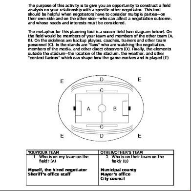
Field Analysis 4n4bm
October 2019 109
Ansys Basic Analysis Guide 306z68
December 2019 51
Harmonic Analysis In Ansys v3s4v
November 2019 52
Ansys Modal Analysis n1h73
November 2019 36More Documents from "Umesh Vishwakarma" p1v3c
Ansys Basic Analysis Guide 306z68
December 2019 51
Ansys Coupled Field Analysis 1y4i3y
October 2019 70
Lic-irda Exam-1 2v2w6o
December 2019 75
Ayurveda Astanga Hridayam.pdf 4q4p2o
October 2019 3,493
Wipro In Pf Settle Form 192t28
December 2021 0