Design Of Experiments. Montgomery Doe u5w6s

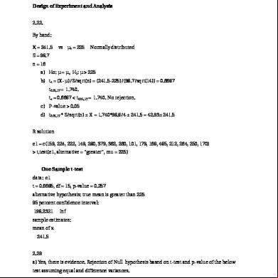
Individual Homework #3 Design of Experiment and Analysis 2.22. By hand: X = 241.5

vs µo = 225

Normally distributed

S = 98.7 n = 16 a) Ho: µ = µo H1: µ > 225 b) to = (X- µ)/S/sqrt(n) = (241.5-225)/(98.7/sqrt(14)) = 0.6687 t0.05, 17 = 1.740. to = 0.6687 < t0.05, 17 = 1.740. No rejection. c) P-value > 0.05 d) t0.05, 17 * S/sqrt(n) ± X = 1.740*98.8/4 ± 241.5 = 42.93± 241.5 R solution e1 = c(159, 224, 222, 149, 280, 379, 362, 260, 101, 179, 168, 485, 212, 264, 250, 170) > t.test(e1, alternative = "greater", mu = 225) One Sample t-test data: e1 t = 0.6685, df = 15, p-value = 0.257 alternative hypothesis: true mean is greater than 225 95 percent confidence interval: 198.2321

Inf

sample estimates: mean of x 241.5 2.29 a) Yes, there is evidence. Rejection of Null hypothesis based on t-test and p-value of the below test assuming equal and difference variances.

> t95 = c(11.176, 7.089, 8.097, 11.739, 11.291, 10.759, 6.467, 8.315) > t100 = c(5.263, 6.748, 7.461, 7.015, 8.133, 7.418, 3.772, 8.963) T-test assuming equal variances > t.test(t95, t100, alternative = "greater", var.equal = TRUE) Two Sample t-test data: t95 and t100 t = 2.6751, df = 14, p-value = 0.009059 alternative hypothesis: true difference in means is greater than 0 95 percent confidence interval: 0.8608158

Inf

sample estimates: mean of x mean of y 9.366625 6.846625 T-test assuming different variances t.test(t95, t100, alternative = "greater", var.equal = FALSE) Welch Two Sample t-test data: t95 and t100 t = 2.6751, df = 13.226, p-value = 0.009423 alternative hypothesis: true difference in means is greater than 0 95 percent confidence interval: 0.8539293

Inf

sample estimates: mean of x mean of y 9.366625 6.846625 b) p-value = 0.009059 Equal variances. p-value = 0.009423 Unequal variances

c) 2.52 ± 1.771*sqrt(4.4/8+2.69/8) = 2.52 ± 1.66. 95% of the time the difference between the thicknesses at 95 and 100 degrees will fall within this interval. d) tfile <- read.csv(file="tem.csv",head=TRUE,sep=",") > tfile T95 T100 1 11.176 5.263 2 7.089 6.748 3 8.097 7.461 4 11.739 7.015 5 11.291 8.133 6 10.759 7.418 7 6.467 3.772 8 8.315 8.963 dotplot(jitter(thickness)~T, data=tfile)

e) Based on normal probability plots normal distribution can be assumed Normal Probability Plots

f)

power.t.test(n=8,delta=2.5,sd=1.88,sig.level=0.05,type="two.sample", alternative =

"two.sided", strict=TRUE) Two-sample t test power calculation n=8 delta = 2.5 sd = 1.88 sig.level = 0.05 power = 0.6964335 alternative = two.sided NOTE: n is number in *each* group g.) library(pwr) pwr.t.test(d=(1.5)/1.88,power=.9,sig.level=.05,type="two.sample",alternative="two.sided") Two-sample t test power calculation n = 34.00074 d = 0.7978723 sig.level = 0.05

power = 0.9 alternative = two.sided NOTE: n is number in *each* group

2.35. a) f1=c(206, 188, 205, 187, 193, 207, 185, 189, 192, 210, 194, 178) f2=c(177, 197, 206, 201, 176, 185, 200, 197, 198, 188, 189, 203) qqnorm(f1, ylab = "Formulation 1") qqline(f1) qqnorm(f2, ylab = "Formulation 2") qqline(f2)

th

th

Points fall more or less on the lines for both formulations between the 25 and 75 percentile justifying the assumption of normal distribution. Also the lines have similar slopes so the assumption of constant variance is met as well. b) No, it does not. No Rejection of Null hypothesis. t = 0.3448 < t0.05, 22 = 1.7171 and p-value = 0.3667

t.test(f1, f2, alternative = "greater", var.equal = TRUE) Two Sample t-test data: f1 and f2 t = 0.3448, df = 22, p-value = 0.3667 alternative hypothesis: true difference in means is greater than 0 95 percent confidence interval: -5.637883

Inf

sample estimates: mean of x mean of y 194.5000 193.0833 c) p-value = 0.3667 d) No it does not. p-value = 0.6482 t.test(f1, f2, alternative = "greater", mu =3, var.equal = TRUE) Two Sample t-test data: f1 and f2 t = -0.3854, df = 22, p-value = 0.6482 alternative hypothesis: true difference in means is greater than 3 95 percent confidence interval: -5.637883

Inf

sample estimates: mean of x mean of y 194.5000 193.0833