E 2546 - 15 5q834
This document was ed by and they confirmed that they have the permission to share it. If you are author or own the copyright of this book, please report to us by using this report form. Report 3b7i
Overview 3e4r5l
& View E 2546 - 15 as PDF for free.
More details w3441
- Words: 13,772
- Pages: 24
Designation: E2546 − 15
Standard Practice for
Instrumented Indentation Testing1 This standard is issued under the fixed designation E2546; the number immediately following the designation indicates the year of original adoption or, in the case of revision, the year of last revision. A number in parentheses indicates the year of last reapproval. A superscript epsilon (´) indicates an editorial change since the last revision or reapproval.
priate safety and health practices and determine the applicability of regulatory limitations prior to use.
1. Scope* 1.1 This practice defines the basic steps of Instrumented Indentation Testing (IIT) and establishes the requirements, accuracies, and capabilities needed by an instrument to successfully perform the test and produce the data that can be used for the determination of indentation hardness and other material characteristics. IIT is a mechanical test that measures the response of a material to the imposed stress and strain of a shaped indenter by forcing the indenter into a material and monitoring the force on, and displacement of, the indenter as a function of time during the full loading-unloading test cycle.
2. Referenced Documents 2.1 ASTM Standards:2 E3 Guide for Preparation of Metallographic Specimens E74 Practice of Calibration of Force-Measuring Instruments for ing the Force Indication of Testing Machines E92 Test Method for Vickers Hardness of Metallic Materials (Withdrawn 2010)3 E177 Practice for Use of the Precision and Bias in ASTM Test Methods E384 Test Method for Knoop and Vickers Hardness of Materials E691 Practice for Conducting an Interlaboratory Study to Determine the Precision of a Test Method E1875 Test Method for Dynamic Young’s Modulus, Shear Modulus, and Poisson’s Ratio by Sonic Resonance E1876 Test Method for Dynamic Young’s Modulus, Shear Modulus, and Poisson’s Ratio by Impulse Excitation of Vibration 2.2 American Bearing Manufacturers Association Standard: ABMA/ISO 3290-1 Rolling Bearings- Balls-Part 1: Steel Metal Balls4 2.3 ISO Standards: ISO 14577-1, -2, -3, -4 Metallic Materials—Instrumented Indentation Tests for Hardness and Material Properties5 ISO 376 Metallic Materials—Calibration of Force-Proving Instruments for the Verification of Uniaxial Testing Machines5
1.2 The operational features of an IIT instrument, as well as requirements for Instrument Verification (Annex A1), Standardized Reference Blocks (Annex A2) and Indenter Requirements (Annex A3) are defined. This practice is not intended to be a complete purchase specification for an IIT instrument. 1.3 With the exception of the non-mandatory Appendix X4, this practice does not define the analysis necessary to determine material properties. That analysis is left for other test methods. Appendix X4 includes some basic analysis techniques to allow for the indirect performance verification of an IIT instrument by using test blocks. 1.4 Zero point determination, instrument compliance determination and the indirect determination of an indenter’s area function are important parts of the IIT process. The practice defines the requirements for these items and includes nonmandatory appendixes to help the define them. 1.5 The use of deliberate lateral displacements is not included in this practice (that is, scratch testing). 1.6 The values stated in SI units are to be regarded as standard. No other units of measurement are included in this standard. 1.7 This standard does not purport to address all of the safety concerns, if any, associated with its use. It is the responsibility of the of this standard to establish appro-
3. Terminology 3.1 Definitions of Specific to This Standard: 2 For referenced ASTM standards, visit the ASTM website, www.astm.org, or ASTM Customer Service at [email protected]. For Annual Book of ASTM Standards volume information, refer to the standard’s Document Summary page on the ASTM website. 3 The last approved version of this historical standard is referenced on www.astm.org. 4 Available from American Bearing Manufacturers Association (ABMA), 2025 M Street, NW Suite 800 Washington, DC 20036, http://www.americanbearings.org.
1 This practice is under the jurisdiction of ASTM Committee E28 on Mechanical Testing and is the direct responsibility of Subcommittee E28.06 on Indentation Hardness Testing. Current edition approved Oct. 1, 2015. Published December 2015. Originally approved in 2007. Last previous edition approved in 2007 as E2546–07ɛ1. DOI: 10.1520/E2546-15.
5 Available from American National Standards Institute (ANSI), 25 W. 43rd St., 4th Floor, New York, NY 10036, http://www.ansi.org.
*A Summary of Changes section appears at the end of this standard Copyright © ASTM International, 100 Barr Harbor Drive, PO Box C700, West Conshohocken, PA 19428-2959. United States
1
E2546 − 15 3.1.9.1 Discussion—The test cycle may include any of the following operations: approach of the indenter towards the test sample, singular or multiple loading, dwell, and unloading cycles. 3.1.10 test data, n—for this practice it will consist, at the minimum, of a set of related force/displacement/time data points. 3.1.11 zero point, n—the force-displacement-time reference point when the indenter first s the sample and the force is zero. 3.1.11.1 Discussion—A course zero point is an approximate value used as part of an analysis to determine a refined value.
3.1.1 stiffness, n—the instantaneous elastic response of the material over the area of with the indenter. 3.1.1.1 Discussion— stiffness can be determined from the slope of line 3 in Fig. 1. 3.1.2 force displacement curve, n—a common plot of the force applied to an indenter and the resultant depth of penetration. 3.1.2.1 Discussion—This plot is generated from data collected during the entire loading and unloading cycle. (See Fig. 1.) 3.1.3 indentation radius [a], n—the in-plane radius, at the surface of the test piece, of the circular impression of an indent created by a spherical indenter. 3.1.3.1 Discussion—For non-circular impressions, the indentation radius is the radius of the smallest circle capable of enclosing the indentation. The indentation radius is normally used as a guide for spacing of indentations. 3.1.4 indenter area function [Λ], n—mathematical function that relates the projected (cross-section) area of the indenter tip to the distance from the apex of the tip as measured along the central axis. 3.1.5 instrument compliance, n—the flex or reaction of the load frame, actuator, stage, indenter, anvil, etc., that is the result of the application of a test force to the sample. 3.1.6 instrumented indentation test (IIT), n—an indentation test where the force applied to an indenter and the resultant displacement of the indenter into the sample are recorded during the loading and unloading process for post test analysis. 3.1.7 nominal area function, n—area function determined from measurement of the gross indenter geometry. 3.1.8 refined area function, n—area function determined indirectly by a technique such as the one described in Appendix X3. 3.1.9 test cycle, n—a series of operations at a single location on the test sample specified in of either applied test force or displacement as a function of time.
3.2 Indentation Symbols and Designations (see Fig. 2 and Table 1): 4. Summary of Practice 4.1 This practice defines the details of the IIT test and the requirements and capabilities for instruments that perform IIT tests. The necessary components are defined along with the required accuracies required to obtain useful results. Verification methods are defined to insure that the instruments are performing properly. It is intended that ASTM (or other) Test Methods will refer to this practice when defining different calculations or algorithms that determine one or more material characteristics that are of interest to the . 5. Significance and Use 5.1 IIT Instruments are used to quantitatively measure various mechanical properties of thin coatings and other volumes of material when other traditional methods of determining material properties cannot be used due to the size or condition of the sample. This practice will establish the basic requirements for those instruments. It is intended that IIT based test methods will be able to refer to this practice for the basic requirements for force and displacement accuracy, reproducibility, verification, reporting, etc., that are necessary for obtaining meaningful test results. 5.2 IIT is not restricted to specific test forces, displacement ranges, or indenter types. This practice covers the requirements for a wide range of nano, micro, and macro (see ISO 14577-1) indentation testing applications. The various IIT instruments are required to adhere to the requirements of the practice within their specific design ranges. 6. Apparatus 6.1 General—The force, displacement and time are simultaneously recorded during the full sequence of the test. An analysis of the recorded data must be done to yield relevant information about the sample. When available, relevant ASTM test methods for the analysis should be followed for comparative results. NOTE 1—The is encouraged to refer to the manufacturer’s instruction manual to understand the exact details of the tests and analysis performed.
1. Increasing test force 2. Removal of the test force 3. Tangent to curve 2 at Fmax
6.2 Testing Instrument—The instrument shall be able to be verified according to the requirements defined in Annex A1 and have the following features.
FIG. 1 IIT Procedure Shown Schematically
2
E2546 − 15
NOTE 1—The symbols shown are the same for pointed and spherical indenters. FIG. 2 Schematic Cross-Section of an IIT Indentation TABLE 1 Symbols and Designations Symbol
Designation
Unit
α
Angle, specific to shape of pyramidal indenter (see Annex A3) Radius of indentation (see 3.1.3) Radius of spherical indenter (see Annex A3) Test force applied to sample Maximum value of F Indenter displacement into the sample Maximum value of h Depth over which the indenter and specimen are in during the force application Permanent recovered indentation depth after removal of test force Surface area of indenter in with material Projected (cross section) area of indenter at depth hc Point of intersection of line 3 with the h axis (see Fig. 1) stiffness Time relative to the zero point
°
a R F Fmax h hmax hc hp
As Ap hr S t
6.2.2 Sample Positioning—The positioning of the sample being tested relative to the centerline of the test force is critical to obtaining good results. The testing instrument shall be designed to allow the centerline of the test force to be normal to the sample surface at the point of indentation. 6.2.3 Indenters—Indenters normally consists of a tip and a suitable holder. The tip should have a hardness and modulus that significantly exceeds the materials being tested. The holder shall be manufactured to the point without any unpredictable deflections that could affect the test results. The holder shall allow proper mounting in the actuator and position the point correctly for the application of the test force. The tip and holder could be a one or multi-piece design. A variety of indenter shapes, such as pyramids, cones, and spheres, can be used for IIT Testing. Annex A3 defines the requirements for the most commonly used indenters. Whenever they are used the requirements of Annex A3 shall be followed. Other indenter shapes can be used provided they are defined in a standardized Method or described in the test report.
µm µm N N µm µm µm µm
µm2 µm2 µm N/µm s
6.2.1 Test Forces/Displacements—The instrument shall be able to apply operator selectable test forces or displacements within its usable range. The controlled parameters can vary either continuously or step by step. The application of the test force shall be smooth and free from any unintended vibrations or abnormalities that could adversely affect the results. The approach, loading, and data acquisition rates shall be controlled to the extent that is required to obtain meaningful estimates of force and displacement uncertainties at the zero point. The estimated uncertainty in the force at the zero point shall not exceed 1 % of the maximum test force (Fmax) or 2 µN, whichever is greater. The estimated uncertainty in the displacement at the zero point should not exceed 1 % of the maximum indenter displacement (hmax) or 2 nm, whichever is greater. If the estimated uncertainty in the displacement at the zero point is larger than both criteria, its value and the influence of its value on reported mechanical properties shall be noted in the test report. See Appendix X1 for information on how to determine the zero point.
NOTE 2—The nominal indenter geometry, as described in Annex A3, may be sufficiently accurate for a given analysis. In many cases, however, a refined area function that more accurately represents the shape of the indenter used may be necessary to provide the desired results (see A3.7).
6.2.4 Imaging Device (Optional)—In applications where it is desirable to accurately locate the indentation point on the sample or observe the indent, an imaging device such as an optical or atomic force microscope may prove helpful. The device should be mounted such that locations can be identified quickly and accurately. 6.3 Data Storage and Analysis Capabilities—The apparatus shall have the following capabilities: 6.3.1 Force/Displacement/Time Measurement—Acquire and store raw force, displacement and time data during each test. 6.3.2 Data Correction—When necessary, conversion of the raw data defined in 6.3.1 to corrected force (F), displacement (h), and time (t) data as defined in 3.2. The conversion shall 3
E2546 − 15 from such features; however, there are exceptions to this rule. The measurements of elastic properties, for example, are significantly more sensitive and require greater spacing than those for plastic properties. It is the responsibility of the operator to exercise caution so that such gradients do not affect the desired results.
consider at least the following parameters: Zero point determination (see Appendix X1), instrument compliance (see Appendix X2) and thermal drift. 6.3.3 Indenter Shape Function—Utilize an appropriate indenter shape function if necessary (see Appendix X3). 6.3.4 Test Result Generation: 6.3.4.1 Perform the desired analysis on the raw or corrected data to obtain useful test results. When available, relevant ASTM or ISO 14577 test methods should be used. 6.3.4.2 Determine indentation modulus (EIT) according to the Test Method defined in Appendix X4 or another method that produces similar results.
8.4 Define the Test Cycle—The test cycle parameters shall be chosen with respect to the following considerations: 8.4.1 The forces generated by the dynamic motion of the indenter mass shall not adversely affect the accuracy of the results. This is particularly true at the point of when the intentionally applied forces are small. 8.4.2 The test cycle force and displacement values used in the test result analysis, except those used for zero point determination, shall be within the verified range of the instrument as reported in A1.7.2.4 and A1.7.2.5.
7. Test Piece 7.1 Surface Finish—The surface finish of the sample will directly affect the test results. The test should be performed on a flat specimen with a polished or otherwise suitably prepared surface. Any contamination will reduce the precision and accuracy of the test. The should consider the indent size when determining the proper surface finish.
8.5 Perform the Test Cycle—The test cycle (see 3.1.9) is performed according to the specifications of the manufacturer or the test method. Force/displacement/time data shall be acquired during each test cycle.
7.2 Surface Preparation—The preparation of the surface shall be done in a way that minimizes alteration of the characteristic of the material to be evaluated.
8.6 Correct the Data—The acquired data shall be corrected according to 6.3.2. The details may be defined by the manufacturer or by a test method.
7.3 Sample Thickness—The thickness of the material to be analyzed may be a critical factor in the ability to obtain the desired results. The test piece thickness shall be large enough, or indentation depth small enough, such that the test result is not influenced by the test piece . The test piece thickness should be at least 10 times the indentation depth or six times greater than the indentation radius; whichever is greater.
8.7 Analyze Results—The corrected data shall be analyzed to obtain the desired test results according to 6.3.4. The details may be defined by the manufacturer or by a test method.
8. Procedure
9.2 The report shall include the following minimum information: 9.2.1 Date and time, 9.2.2 Reference to this practice, 9.2.3 Description of instrument—mfg., model, etc., 9.2.4 Shape and material of the indenter used, 9.2.5 Temperature, 9.2.6 Test sample description, 9.2.7 Description of test cycle, 9.2.8 Method of zero point determination, 9.2.9 Reference to analytic method used, including values of any model dependent parameters, 9.2.10 Number of tests and results, 9.2.11 Details of any occurrence that may have affected the results, and 9.2.12 Define the units of the test results.
9. Report 9.1 The report shall include sufficient information about the test cycle, indenter, sample and analysis method used to allow the final results to be reproduced.
8.1 Prepare Environment—The test should be carried out within the temperature range defined by the manufacturer. Prior to performing any tests the instrument and the test sample shall be stabilized to the temperature of the environment. Temperature change during each test should be less than 1.0°C. The test environment shall be clean and free from vibrations, electromagnetic interference, or other variations that could adversely affect the performance of the instrument. Testing done outside the specified limits is allowed; however, all deviations shall be specified on the test report. 8.2 Mount Specimen—The sample shall be rigidly ed and the test surface shall be positioned normal to the centerline of the test force. NOTE 3—Sample fixtures may add to the compliance of the instrument. The should consider the impact of this undesirable effect.
NOTE 4—It is also frequently desirable to describe the location of the indentation on the test piece as part of the report.
8.3 Select Test Location—The results of indentation tests will be adversely affected if the properties being measured vary within the volume of material being deformed. Extreme conditions would be caused by the presence of free surfaces such as edges, voids and other indentations. For many materials it is sufficient to locate the test at least six indent radii away
10. Keywords 10.1 force displacement curve; indentation hardness; indentation modulus; indenter shape function; instrument compliance; instrumented indentation; zero point
4
E2546 − 15 ANNEXES (Mandatory Information) A1. INSTRUMENT VERIFICATION
shall provide documentation confirming that the verification results would be within the tolerance if the force were applied in the test direction. A1.3.2.4 If the force calibration is assumed to be independent of indenter position, the manufacturer shall show that this is the case.
A1.1 Scope A1.1.1 This annex specifies procedures for verification of testing machines that conform to the requirements defined in this practice. The annex describes a direct verification procedure for checking the main functions of the testing machine and an indirect verification procedure suitable for assessing the overall performance of the testing machine. The indirect procedure is used as part of the direct procedure and for the periodic routine checking of the machine in service. This annex does not cover verification procedures for specific indenter geometry; such procedures are presented in Annex A3 Indenter Requirements. The manufacturer’s recommendations concerning instrument calibration and verification should be used as long as they do not conflict with the specifications of this annex.
A1.3.3 Displacement Verification—Each displacement range of the instrument shall be verified as described below. A1.3.3.1 At least ten verification lengths shall be chosen so as to span evenly the defined displacement range. The measurement of each verification length shall be repeated three times. Every measurement shall be within 1 % or 2 nm of its nominal value, whichever is greater. If the 2nm tolerance is used the maximum indenter displacement (hmax) shall be accurate to within 5 % of the stated value. The verified displacement range of an instrument shall be defined as the range of lengths from the minimum verified length to the maximum verified length. A1.3.3.2 The device used for displacement verification shall be accurate to within 0.25 % or 1 nm of each verified length, whichever is greater. Methods of producing lengths for verification include: (1) Laser interferometers, (2) Film thickness standards, and (3) Independent actuator or transducer.
A1.2 General Conditions A1.2.1 Direct and indirect verification procedures shall be carried out at a temperature of 23 6 5°C. NOTE A1.1—For both verification and operation, thermal stability of the instrument is important. During any verification procedure, reasonable care should be taken to ensure that the temperature of the instrument and its immediate environment are kept at a constant temperature, preferably to within a 0.5°C range over the course of the verification procedure or test.
A1.3 Direct Verification
A1.3.4 Timing Verification—The time required for a test segment at least ten seconds in duration shall be verified by an independent timing device. The difference between the time reported by the test equipment and that measured by an independent timing device must be less than 1.0 seconds. A hand-operated, non-traceable, stopwatch is sufficient for this verification.
A1.3.1 Direct verification requires assessment of: (1) Force, (2) Displacement, and (3) Timing. If available, the devices used for force and displacement verification shall be traceable to National Standards. A1.3.2 Force Verification—Each force range of the instrument shall be verified as described below. A1.3.2.1 At least ten verification forces shall be chosen that evenly span the defined force range. The measurement of each verification force shall be repeated three times. Every measurement shall be within 1 % or 2 µN of its nominal value, whichever is greater. When the 2 µN tolerance is used the maximum test force (Fmax) shall be accurate to within 5 % of the stated value. The verified force range of an instrument shall be defined as the range of forces from the minimum verified force to the maximum verified force. A1.3.2.2 The device used to forces shall be accurate to within 0.25 % or 1 µN of each verification force, whichever is greater. Examples of techniques for force verification include: (1) Measuring by means of an elastic proving device in accordance with Practice E74 (class A), or ISO 376 (class 1), (2) Balancing against a force, applied by means of calibrated masses, and (3) Measuring by means of an electronic balance. A1.3.2.3 If the verification force is applied in the opposite direction from the force used during a test, the manufacturer
A1.4 Indirect Verification A1.4.1 An independent indirect verification shall be performed for each force range of the instrument. Indirect verification is intended to monitor the total performance of the instrument including force and displacement calibrations, machine compliance, indenter shape function, method of zeropoint determination, and the analysis procedures. Therefore, these parameters shall remain fixed during indirect verification. A1.4.2 Procedure—Indirect verification requires determining the indentation modulus, EIT, of two materials of known Young’s modulus. The two material’s Young’s modulus shall differ by at least a factor of two. Test blocks that comply with Annex A2 of this practice, should be used. NOTE A1.2—The Test Method defined in Appendix X4 is recommended for this procedure.
A1.4.2.1 On each material, five tests shall be performed within each of the following force ranges: 5
E2546 − 15 A1.6.2.5 When the correction for machine compliance is changed.
(1) A maximum force within the lower 25 % of the verified force range, and (2) A maximum force within the upper 25 % of the verified force range. A1.4.2.2 The instrument is considered verified if ninety percent of the values of indentation modulus reported by the test equipment match the nominal Young’s modulus, or the dynamic Young’s modulus, value assigned to the material to within 65 %.
NOTE A1.5—If the correction for machine compliance is known to change in a predictable way, that is, as a function of mounting type or sample position, the machine compliance correction may be changed according to a pre-established algorithm. An indirect verification is not required after such a change.
A1.6.2.6 Following the replacement of a component in either the force or displacement measurement system, provided that the manufacturer can show that such a replacement does not affect the force or displacement calibration of the complete machine.
A1.4.3 Failure of the Indirect Verification—When the results of the indirect verification are unsatisfactory, the manufacturers’ guidelines for troubleshooting should be followed, and the indirect verification repeated. If the results are still not satisfactory, the instrument fails indirect verification.
NOTE A1.6—It is recommended that the indirect verification process be used to determine the indenter shape function for a specific indenter.
A1.6.3 Routine Checking—Routine checking shall be performed: A1.6.3.1 Every day that the instrument is used, A1.6.3.2 When an indenter is changed, and A1.6.3.3 After changes in hardware that may affect the machine compliance.
A1.5 Routine Checking A1.5.1 Routine checking shall be used according to the schedule defined in A1.6.3 to monitor the performance of the instrument. A1.5.2 Procedure—Routine checking requires performing at least three tests on a single material of known indentation modulus. The test parameters, such as maximum force and displacement, should be similar to those that will be used until the next routine check. Eighty percent of the values of indentation modulus reported by the instrument shall match the expected value to within 65 %.
A1.6.4 Verification Flowchart—A flowchart showing guidelines for verification of the various components is shown in Fig. A1.1. A1.7 Reporting Results for Verifications and Routine Checking
NOTE A1.3—The test method used may require additional testing on test blocks or other reference materials unique to the method.
A1.7.1 Results from all direct and indirect verifications, including out-of-tolerance data, shall be maintained in a log associated with the instrument.
A1.5.3 Failure of Routine Checking—When the results of routine checking are unsatisfactory, the manufacturers’ guidelines for troubleshooting should be followed, and the routine check repeated. If the results are still not satisfactory, the instrument fails routine checking.
A1.7.2 Direct Verification Report—Reporting for a direct verification shall include at least the following information: A1.7.2.1 Reference to this standard, A1.7.2.2 Identification data for the machine, A1.7.2.3 Environmental temperature and humidity, A1.7.2.4 Verified force range of the instrument, as well as verification forces used and measured values for those forces (see A1.3.2 of this annex), A1.7.2.5 Verified displacement range of the instrument, as well as verification lengths used and measured values for those lengths (see A1.3.3 of this annex), A1.7.2.6 Identification of devices used for force and displacement verification, including any relevant traceability information, A1.7.2.7 Results of timing verification including nominal time of the test segment and measured time, and A1.7.2.8 Name of the verification laboratory and date of verification.
A1.6 Verification Schedule A1.6.1 Direct Verification—Direct verification shall be performed: A1.6.1.1 When the instrument is first certified to comply with this standard, A1.6.1.2 Following a major repair or overhaul of the instrument, including replacement of a component in the force or displacement system, except as described in A1.6.2 of this annex, and A1.6.1.3 When the instrument fails indirect verification as defined in A1.4 of this annex. NOTE A1.4—It is recommended that direct verification be performed upon installation of an instrument at a new location and at intervals not to exceed three years. Instruments intended for portable use cannot easily be directly verified at each location; therefore they should be verified at a known stable location.
A1.7.3 Reporting for Indirect Verification—Reporting for an indirect verification shall include all of the information required by standard reporting as described in Section 9. Test sample description shall include the nominal dynamic Young’s modulus for the test materials.
A1.6.2 Indirect Verification—Indirect verification shall be performed: A1.6.2.1 Following direct verification, A1.6.2.2 After any relocation of the instrument, except for instruments designed specifically for portable use, A1.6.2.3 At intervals not to exceed one year, A1.6.2.4 When the machine fails routine checking as defined in A1.6.3 of this annex, and
A1.7.4 Documentation of Routine Checking—A formal report for routine checking is not required. However, it is recommended that a log of these results be maintained. 6
E2546 − 15
FIG. A1.1 Verification Flowchart
A2. STANDARD REFERENCE BLOCKS
A2.1 Scope
above a certain force, or unacceptable scatter in indentation results below a certain indentation force as the result of surface roughness or small-scale nonhomogeneities.
A2.1.1 This annex specifies requirements for the production and certification of standard reference blocks for use in the indirect verification of instrumented indentation instruments, as described in A1.6.2 of this practice.
NOTE A2.1—These minimum and maximum values for force or displacement will in general be indenter-specific. For example, maximum loads for blocks of brittle material may be much higher for large-radii spheres than for Berkovich tips.
A2.2 General Requirements
A2.3 Material Selection
A2.2.1 Standard reference blocks shall be manufactured from materials with known values of dynamic Young’s modulus, E, and Poisson’s ratio, ν, each determined to an accuracy better than 1.0 %.
A2.3.1 Materials for standard reference blocks should have the following characteristics: A2.3.1.1 A well-known, uniform composition, A2.3.1.2 An amorphous or single crystal structure or known grain size distribution, A2.3.1.3 Isotropic elastic properties, A2.3.1.4 A chemically stable surface, A2.3.1.5 A melting or glass transition temperature well above room temperature, and
A2.2.2 Each test block shall be provided with certified values of dynamic Young’s modulus and Poisson’s ratio. Instrumented indentation tests shall be used to determine a usable range of depth or load for each block. Examples of material characteristics that might limit the range of appropriate indentation force include the cracking of a brittle material 7
E2546 − 15 for each test block, and the force or depth range over which the blocks will perform satisfactorily. This information depends not only on the particular test block material, but on block preparation as well.
A2.3.1.6 Little or no pile-up of material about the perimeter of the indentation site. A2.4 Manufacture of Reference Blocks A2.4.1 Test Surface Orientation—Reference blocks shall be manufactured in such a way that the test surface can be presented perpendicular to the indenter axis within 0.5 degrees. For specimens that are intended to be placed with their bottom surface (that surface opposite the test surface) on a specimen mounting plate, this requirement shall be met by achieving the necessary 0.5 degree parallelism between top and bottom surfaces. For specimens that are to be mounted by their sides (that is, a cylindrical reference block clamped in a V-shaped vise), the side surfaces shall be perpendicular to the test surface to within 0.5 degrees.
A2.5.3 The test block manufacturer shall confirm that the elastic properties of the block at its test surface do not deviate from the bulk values by more than 5 %, due to, for example, any grinding, polishing or annealing processes used in the preparation of the blocks. Methods to accomplish this could include, for example, test indentation by the manufacturer or measurement of surface elastic properties by surface acoustic wave methods. A2.5.4 Surface roughness shall be measured on each polishing batch, or on each deposition batch, in the case of a deposited test surface layer. The manufacturer shall report the method used for surface roughness determination.
A2.4.2 Test Surface Finish—Test surface roughness can seriously degrade the accuracy and reproducibility of indentation test results. Therefore, reference blocks should be prepared in such a way that the test surface presented is as smooth as is possible for a given material. An acceptable value of average surface roughness, RA, for many applications is RA ≤ 10 nm measured over a 10 µm trace. Blocks intended specifically for very-low-force verification will require lower roughness levels. For guidelines on the preparation on metallographic specimens, see for example Guide E3.
A2.5.5 Each block must be marked with it’s own a serial number or letters. The markings may be on the top or side of the block. If the marking is on the side of the block, the markings shall be upright when the test surface is the upper surface. A2.6 Certification Report A2.6.1 The report for each test block shall at contain the following minimum information: A2.6.1.1 The name of the laboratory certifying the block, A2.6.1.2 The certified values for dynamic Young’s modulus, E, and Poisson’s ratio, ν, along with the uncertainty of each, A2.6.1.3 The method by which E and ν were determined, including identification of the equipment used and relevant traceability information for that method and equipment, A2.6.1.4 The serial number of the block, A2.6.1.5 The date of certification, A2.6.1.6 The regions of the block surface that is not available to the for indentation; examples of such regions include areas that are too close to an edge, or regions that were used by the manufacturer for indentation or other quality control testing that might have altered the surface properties, A2.6.1.7 The indenter geometries for which the block is appropriate, and range of indentation force or depth over which the block may be expected to perform satisfactorily for each specified indenter geometry, A2.6.1.8 The surface roughness of the test surface, including a precise definition of the roughness quantity reported and a description of how it was determined, and A2.6.1.9 An expiration date, if one is appropriate for a given test material.
A2.4.3 Reference Block Compliance—In some cases, the reference block may consist of a smaller piece of test material in a larger, integral mount, or a deposited surface layer on a substrate. If this is the case, care must be taken by the test block manufacturer to ensure that the stiffness of that integral mount or substrate is sufficiently high that its compliance does not significantly affect the measured elastic properties of the test material. A2.5 Certification Procedure A2.5.1 The test block manufacturer shall determine both the dynamic Young’s modulus and Poisson’s ratio for the test block material, each to within 1.0 % accuracy, using the current versions of Test Methods E1875 or E1876. This process may be performed either on each block or on a larger batch of material prior to sectioning or separation of individual test blocks. If such “batch certification” is performed, the manufacturer shall confirm, by testing a limited but statistically significant number of specimens that blocks from various locations within the original batch all meet the general requirements given in A2.2. A2.5.2 The test block manufacturer shall determine general guidelines concerning which indenter geometry’s are suitable
8
E2546 − 15 A3. INDENTER REQUIREMENTS
A3.1 Scope A3.1.1 This annex will define the requirements for the various indenters typically used for IIT. The physical dimensions and manufacturing tolerances of the most common indenters will be defined along with the requirements for certification. A3.2 General Requirements A3.2.1 The indenters used for IIT can be many different shapes to suit the test method used. All indenters shall meet the following requirements: A3.2.1.1 The part of the indenter that s the sample shall be made from a hard material and have a defined shape. They can be a one piece or multi-piece design. A3.2.1.2 The surface of the indenter that s the sample shall be highly polished and free from chips, pits, contamination and any other imperfections that may affect its final use. The surface shall be observed under a microscope with a magnification of least 50×. FIG. A3.1 Angle of the Vickers Diamond Pyramid
NOTE A3.1—Spherical indenters that meet the requirements of ABMA/ ISO 3290-1 Grade 24 do not have to be inspected optically.
A3.2.1.3 Each indenter shall have a unique serial number. In the case of a ball indenter, the holder only shall be serialized. The serial number shall be marked on the indenter or holder in a manner that cannot be easily removed. Indenters that are too small to be easily marked shall have the serial number marked on its container. A3.2.1.4 The indenters shall be measured to their conformance to the dimensional requirements. A nominal indenter area function at the maximum usable indentation depth shall be calculated based on the actual dimensions of the indenter. A3.2.1.5 Spherical indenters that are part of a batch of balls from a lot that meet the requirements of ABMA/ISO 3290-1 Grade 24 do not have to be individually measured or have a indenter area function determined. A3.2.1.6 Indenters for use at indentation depths ≤0.006 mm shall have their area function defined over the relevant indentation depth range of use per A3.7.
A3.4 Three Sided Pyramidal Pointed Indenters A3.4.1 There are three commonly used three sided pyramidal indenters used for IIT. They shall meet the following requirements: A3.4.1.1 Berkovich and Modified Berkovich—There are two types of Berkovich pyramidal diamond indenters in use. The original Berkovich indenter was designed to have the same surface area as a Vickers indenter at any given indentation depth. The modified Berkovich indenter is more commonly used and has the same projected area as a Vickers indenter at any given indentation depth. The angles and tolerances for a Berkovich indenter shall meet the angle and tolerance requirements defined in Fig. A3.3. A3.4.1.2 Cube Corner—The angles and tolerances for a cube corner indenter shall meet the angle and tolerance requirements defined in Fig. A3.3. A3.5 Spherical Ball Indenters A3.5.1 The ball shall be harder than the test piece. Carbide balls with hardness not less than 1500 HV10 and having the chemical composition defined in Table A3.1 are recommended.
A3.3 Vickers Indenters A3.3.1 Vickers indenters that are used for IIT are similar to the indenters defined in Test Methods E384 and E92. They shall meet the following requirements: A3.3.1.1 The angle between the opposite faces of the vertex of the diamond pyramid shall be (136 6 0.3°) (see Fig. A3.1). A3.3.1.2 The angle between the axis of the diamond pyramid and the axis of the indenter holder (normal to the seating surface) shall not exceed 0.5°. A3.3.1.3 The four faces should meet at a sharp point. The maximum permissible length of the line of conjunction, c, between opposite faces shall be 0.001 mm (see Fig. A3.2).
A3.5.2 The balls shall meet the tolerance defined in Table A3.2. It is permissible to certify their compliance to the requirements of this section by using batch inspection techniques. NOTE A3.2—Balls that conform to ABMA/ISO 3290-1 Grade 24 satisfy these requirements.
A3.6 Spherical Tipped Conical Indenters A3.6.1 Indenters with a spherical tipped cone shape are useful for many applications. These indenters are normally made from diamond but may also be made from other 9
E2546 − 15
FIG. A3.2 Line of Conjunction at the Tip of the Indenter, Schematically TABLE A3.2 Tolerances for Ball Indenters Ball Indenter Diameter, mm
Tolerance, mm
10 5 2.5 1 0.5
±0.005 ±0.004 ±0.003 ±0.003 ±0.003
TABLE A3.3 Tolerances for Sphero-Conical Indenters Feature Average Radius (Rav) # 0.050 mm 0.500 > Rav > 0.050 mm Cone included angle (2α) 120° 90° 60° Cone flank angle (α) to centerline of mount 60° 45° 30° Point of intersection of cone flanks to centerline of mount
α = 65.03° 6 0.3° for Berkovich indenter α = 65.27° 6 0.3° for modified Berkovich indenter α = 35.26° 6 0.3° for corner cube indenters
Tolerance ±0.25 Rav ±0.10 Rav ±5° ±5° ±5° ±5° ±2.5° ±2.5° within 0.01 mm
FIG. A3.3 Angle of the Berkovich and Cube Corner Indenters TABLE A3.1 Carbide Ball Chemical Composition Chemical Cobalt (Co) Total other carbides Tungsten Carbide (WC)
point of first should not vary by more than a factor of two from the average radius, that is, 0.5 < R(h)/Rav < 2.
Percent 5.0 to 7.0 % 2.0 % balance
NOTE A3.3—Geometry suggests that the depth of spherical cap hs on a cone of included angle 2α and radius Rav is given by: h s 5 R av~ 1 2 sin ~ α !!
(A3.1)
A3.6.3 In practice, there is a gradual transition from spherical cap to cone geometry, which is hard to specify. Given this and the uncertainties in Rav and α allowed (see Table A3.3), caution should be exercised whenever the depth exceeds 0.5 hs.
materials, for example, ruby, sapphire or hard metal as long as the material is significantly harder than the sample being tested. They are intended to indent only with the spherical tip. The characteristics of spherical tipped conical indenters shall be as given in Table A3.3.
A3.7 Indenter Area Function
A3.6.2 The instantaneous radius of curvature (R(h)) of the spherical cap at any indentation depth h measured from the
A3.7.1 Most of the results determined from an IIT test are based on the projected area of the indenter. However, 10
E2546 − 15 A3.8.1.1 Date of verification, A3.8.1.2 ing laboratory, A3.8.1.3 Description of indenter, A3.8.1.4 Reference to this practice, A3.8.1.5 Unique serial number, A3.8.1.6 Geometrical data with an uncertainty statement, A3.8.1.7 Nominal area function and maximum valid depth, A3.8.1.8 Refined area function (if determined) and valid depth range, and A3.8.1.9 Description of technique used to determine refined area function (if determined).
usually, only the indentation depth is measured. When the maximum depth, hc, is less than 6 µm, the relationship between depth and projected area may be significantly different from that predicted by the nominal area function. Therefore, when the indenter is used in this regime, a refined area function shall be determined. Either of the following techniques is recommended: A3.7.1.1 A direct measurement method using a traceable atomic force microscope (AFM). A3.7.1.2 Indirectly by utilizing indentations into a material of known Young’s modulus (see Appendix X3). A3.8 Report A3.8.1 At least the following items shall be included in the report:
APPENDIXES (Nonmandatory Information) X1. ZERO-POINT DETERMINATION
by 5 mN. As a second example, there may be a linear relationship between force and displacement before due to the stiffness of the testing instrument, as revealed by a linear fit to the pre- data. If that is the case, then all F0 values may be reduced by the amount (mx + b), where m and b are the slope and intercept of the linear fit, and x is the displacement data. X1.2.3 Now let us consider the option of repeated differentiation. For the example of the load cell with an offset of 5 mN, the first derivative of force (F0) with respect to displacement will yield pre- force data that are centered about zero. For the example of a testing instrument with a linear relationship between force and displacement before , the second derivative will produce the same result. It should be noted that differentiation may be accomplished by several means, including numerical and electronic. The advantage of repeated differentiation is that it can be done with no a priori information regarding the pre- functional relationship between force and displacement. (Or more simply, one doesn’t need to know the stiffness and offset of the testing instrument.) The disadvantage is that repeated numerical differentiation of experimental data tends to produce series that are progressively more “scattered.” X1.2.4 Optional—Create F2 by summing F1 over a sliding window of N points. Although this step is optional, it can significantly increase the sensitivity to because gradual changes from the baseline (zero) are accumulated. The first N–1 entries in F2 are invalid. The Nth value for F2 is calculated by summing the first N values of F1. The (N+1)st value for F2 is calculated by summing the second through the (N+1)st values of F1, and so forth. Note that N should be large enough to cover several cycles if there is any periodicity in the pre- data. (A single value of N should be chosen for a particular combination of instrument and data acquisition rate; that is, once chosen, N should not change frequently.)
X1.1 Scope X1.1.1 This appendix describes two analyses by which one may determine the zero point for an individual instrumented indentation test and the corresponding uncertainties in force and displacement. Because this practice pertains only to quasistatic instrumented indentation testing of time-invariant materials, determination of zero-point with respect to time is not essential and is not addressed. Asg t = 0 to the first (F, h, t) triple is common practice. X1.1.2 The analyses in this appendix are intended to be used post-test to assign the zero point for the purpose of data analysis. For a variety of reasons, it may be necessary to assign a coarse zero point during the actual experiment. X1.1.3 Some comments about the uncertainty of the zero point at very low forces are given in X1.4. X1.2 Procedure A X1.2.1 This procedure may be applied if both force and displacement are acquired continuously throughout approach and . It is not appropriate for systems, which apply a specific preload before initiating acquisition of force, displacement, and time data. It should be noted at the outset that this procedure calls for calculating new data series based on the original force data. These series are only for the purpose of determining the zero point. The original force data series will be denoted F0. Subsequent series are denote with incremented subscripts: F1, F 2, and F3. X1.2.2 Create F1 by adjusting F 0 so that pre- forces are centered about zero. At least two options are available for accomplishing this task: compensation with a known analytic function or repeated differentiation. As an example of the compensation option, a load cell may have some known offset of 5 mN, and so force readings before are scattered about that value. Consequently, all F0 values should be reduced 11
E2546 − 15 of revolution. Consequently, the initial portion of the loading curve often follows the mechanics originally formulated by Hertz, that is, F = 4/3Er R1/2D3/2, where F is load, Er is reduced modulus, R is combined radius of curvature (equal to the apical radius of curvature of the tip in the case of indentation into a flat specimen), and D is sum of tip and sample deformation. This equation is expected to hold true in the absence of appreciable attractive surfaces forces, up to the onset of plastic deformation, assuming that the shape function of the tip does not deviate from the rounded geometry over the range of wholly elastic deformation. A note of caution: the Hertz equation applies rigorously to the parabolic geometry but only approximately to the spherical geometry. Nevertheless, the spherical geometry is virtually identical to the parabolic geometry as long as the radius remains much less than the apical radius of curvature of the tip. Furthermore, nearly all materials yield before these two geometries deviate significantly.
X1.2.5 Calculate the standard deviation in F1 (or F2 if created) before , σ. X1.2.6 Create F3 by dividing F1 (or F2 if created) by σ. It should be noted that the series F3 is dimensionless and has the meaning of multiples of the pre- noise (as quantified by the standard deviation) in either F1 or F2. X1.2.7 Tag the data point S2 to be the first point for which F3 exceeds 10. X1.2.8 Tag the data point S1 to be the last point before S2 for which F3 is less than 1. X1.2.9 Set the zero point, S, to be the first point after S1 for which F3 is greater than 4. NOTE X1.1—S2, S1, and S may all be interpolated points.
X1.2.10 Calculate the uncertainty in force due to the uncertainty in the assignment of the zero point to be half the change in F0 between S1 and S2. X1.2.11 Calculate the uncertainty in displacement due to the uncertainty in the assignment of the zero point to be half the change in displacement between S1 and S2.
X1.3.2 This procedure for eliminating the zero point error involves fitting the Hertz equation to the initial portion of the loading curve in order to determine the shift in displacement origin that minimizes the fit residuals. It is appropriate both for instruments that acquire pre- data and instruments that commence the load cycle from a small intentional preload. Because this procedure requires data within the range of wholly elastic deformation, the instrument must be capable of making measurements at very low stresses, through a combination of adequate force and displacement sensitivities and sufficiently large radius of curvature of the apex of the tip.
X1.2.12 Example of Using Procedure A—Table X1.1 provides force-displacement data through approach and between a diamond indenter and polycarbonate. The following steps are used to determine the zero point and the associated uncertainties with respect to both force and displacement. X1.2.12.1 Step A1—Using the first 108 data points (data up to –20 nm), the force-displacement data are fit to a line. This yields a slope of –0.00409 and an intercept of 0.17962. Using this line, the series F1 is calculated so that pre- force values are about zero. These compensated data are plotted in Fig. X1.1. X1.2.12.2 Step A2—The series F2 is created using a window size of 20 data points. The first 19 entries in F2 are invalid. The 20th entry in F2 is the sum of the first 20 values of F1. The 21st entry in F2 is the sum of values 2 ~ 21 of F1, and so forth. X1.2.12.3 Step A3—The standard deviation in F2 is calculated over the first 108 points to be 0.1045 µN. X1.2.12.4 Step A4—The series F3 is created by dividing all values in the series F2 by 0.1045 µN. X1.2.12.5 Step A5— S2, S1, and S are all determined as described in the procedure and plotted in Fig. X1.1. X1.2.12.6 Step A6—The uncertainties with respect to force and displacement due to the assignment of the zero point are calculated to be 60.085 µN, and 60.81 nm, respectively.
X1.3.3 The as-acquired load-displacement curve may possess a residual slope (for example, uncompensated spring force) and a residual offset (for example, constant offset in the load cell output) in its baseline. Identify a portion of the load-displacement curve known to represent out-of- data. This portion may correspond to pre- data or data obtained after fully extracting the tip from the specimen when completing the unloading process. Once identified, perform a linear curve fit to the selected out-of- data and subtract the resulting fit equation (of y = mx + b form, where y is force and x is displacement) from the entire data set in order to obtain a new baseline that is statistically flat and without offset. X1.3.4 Make a best-guess manual correction to the displacement zero point if it is obvious that a significant shift along the displacement axis would result in a substantially improved displacement zero point.
X1.3 Procedure B
X1.3.5 Inspect the initial portion of the loading curve to identify the onset of plasticity. In some instances, the onset of plasticity is signaled by a displacement excursion (pop-in) in the case of load control instruments or a sudden load drop in the case of displacement control instruments. In other instances, the onset of plasticity is not so dramatic but a point where the Hertz equation no longer can hold true still may be evident. Use these observations as a guide for choosing the range of data to be included in the subsequent curve fitting procedure. If available, also include a segment of pre- and potentially pre- data leading up to the best-guess point of initial . Ideally, the chosen range of data is
X1.3.1 Indenter tips generally possess a rounded apex that can be described geometrically as a sphere or as a paraboloid TABLE X1.1 Indentation Depth at 1 µN for Various Combinations of Reduced Modulus (Er) and Indenter Radius of Curvature as Estimated from Hertz Theory Er (GPa) 0.1 1 10 100
Radius of Curvature of Indenter (nm) 10
100
1000
178 38.3 8.25 1.78
82.5 17.8 3.83 0.825
38.3 8.25 1.78 0.383
12
E2546 − 15
NOTE 1—Uncertainty in force is 60.085 µN; uncertainty in displacement is 60.81 nm. FIG. X1.1 Determination of Zero Point (S) for a Test on Polycarbonate
establishing the best choice of fitting window proved to be unsuccessful. Visual comparison clearly indicated that the correlation coefficient was impacted more by the number of points included within the fitting window than by the quality of fit over the range of included points.
comprised of a segment of pre- data followed by in- data leading up to the onset of plasticity. X1.3.6 If the onset of plasticity is clearly evident, simply use a suitable nonlinear curve-fitting algorithm (for example, Levenberg-Marquardt) to fit the Hertz equation to the data range selected in step X1.3.5. For the purpose of curve fitting, the Hertz equation can be parameterized as F = C(D+Ds)3/2, where C is a fit coefficient and Ds is a rigid displacement shift. A note of caution: the chosen algorithm must be able to handle domain errors that might arise from attempts to compute the 3/2 power of a negative number. The algorithm employed for the example given below involves defining a fitting window specified by left-side and right-side displacement cutoffs. The algorithm performs curve fitting iteratively, correcting the displacement values after each cycle by the newly found Ds, until Ds finally takes on a value of zero (or near zero as defined by a suitable convergence criterion). The total correction to the displacement zero point is the sum of Ds from each cycle and the manual correction made in step X1.3.4. The algorithm described here is effective at pulling the data to the correct position within the fitting window if two initial conditions are met: X1.3.6.1 The first cycle is seeded by data clearly representing falling within the fitting window; and X1.3.6.2 The position of the zero point after manual correction is in the vicinity of the fitting window.
X1.3.8 The algorithm described here estimates uncertainties in force and displacement zero points by computing root-meansquare errors from the comparison of the fully corrected experimental curve to the best-fit theoretical curve. Any fully corrected experimental point with load and displacement values at zero or positive are included in the uncertainty analysis, as long as it falls within an uncertainty radius defined as some fraction of the right-side displacement cutoff. X1.3.9 Example of Using Procedure B—The loaddisplacement data (collected under load control) used in this example is identical to that of the example given in Procedure A. X1.3.9.1 Step B1—The residual slope in the out-of- load signal is eliminated by subtracting the linear fit to the loading data, over the range of –47.1 to –15 nm, from the entire load-displacement curve. X1.3.9.2 Step B2—It is evident that adding 10 nm to all displacement values would markedly improve the displacement zero point. X1.3.9.3 Step B3—A fitting window with a left-side displacement cutoff of –5 nm and a right-side displacement cutoff of 10 nm is chosen for the Hertzian curve-fitting procedure. The best-fit Ds is positive 12.34 nm relative to the as-acquired load-displacement curve (compared to 11.61 nm for Procedure A). The uncertainties associated with the zero point are estimated as 60.065 µN and 60.43 nm (compared to 60.085 µN and 60.81 nm for Procedure A) for an uncertainty radius of 25 % of the right-side displacement cutoff (or 2.5 nm). ing for the uncertainties, Procedures A and B are in good agreement. It is noted, however, that Procedure B is more likely to suppress the impact of non-ideal behavior often observed at the shallowest of depths in comparison to Procedure A.
X1.3.7 Repeating step X1.3.6 as a function of right-side displacement cutoff may be necessary if a range of data representing wholly elastic displacements is not evident. As a general observation, both C and Ds often remain flat over a range of right-side displacement cutoffs, but change rapidly when the right-side displacement cutoff is too small (owing to extremely ill-defined geometry, effects caused by chemical contaminants, influence of instrument noise, etc.) or too large (owing to the inclusion of data representing plastic deformation). A suitable choice for the right-side cutoff is one that falls within the range of stable C and Ds. It is noted that attempts to utilize the correlation coefficient as a metric for
13
E2546 − 15
FIG. X1.2 As-acquired Force-Displacement Curve for Polycarbonate
FIG. X1.3 Force-Displacement Curve After Correcting for Residual Slope in Out-of- Load Signal
X1.3.9.4 Step B4—Because the onset of plasticity for polycarbonate did not involve a sudden displacement excursion, a
more thorough fitting analysis was conducted by examining the evolution of best-fit Ds and C over a range of right-side
14
E2546 − 15
FIG. X1.4 Force-Displacement Curve After Manual Shift of Zero Point
FIG. X1.5 Hertzian Fit to Force-Displacement Curve and Fitting Statistics
displacement accuracies at very small values, the radius of curvature of the indenter, the elastic modulus of the test specimen, the presence of adsorbed water, other sources of attractive forces, etc. Table X1.1 displays estimates of indentation depth at 1 µN (a very low test force) for various combinations of reduced modulus and indenter radius of curvature. As can be seen from the table, a compliant sample in combination with a sharp indenter could result in a large
displacement cutoffs. Plots of these two parameters against right-side displacement cutoff indicate that the curve-fitting results of X1.3.9.3 are adequate for defining the zero point. X1.4 Uncertainty X1.4.1 For applications using very low test forces the uncertainty in the displacement at the zero point is highly dependent on force and displacement noise floors, force and 15
E2546 − 15
NOTE 1—Region of low gradient (10 nm [Ds] 13 nm) indicates range of stable curve fits with respect to Hertz equation. FIG. X1.6 Best-Fit Ds for Various Right-Side Displacement Cutoffs, with Left-Side Displacement Cutoff Fixed at –5 nm
absolute uncertainty in the displacement at the zero point if the force noise floor of the instrument is not substantially better
than 1 µN.
16
E2546 − 15
NOTE 1—Region of low gradient is consistent with range of stable values of Ds found in Fig. X1.5. FIG. X1.7 Best-Fit C for Various Right-Side Displacement Cutoffs, with Left-Side Displacement Cutoff Fixed at –5 nm
X2. DETERMINATION OF INSTRUMENT COMPLIANCE
C∆ = correction to original value of Cf*. Cf = new value for instrument compliance.
X2.1 Scope X2.1.1 This appendix describes a procedure by which instrument compliance may be determined for the instrument described in Section 6 of this practice.
X2.4 General Conditions X2.4.1 The instrument and procedure shall comply with Sections 6 and 8 of this practice, respectively. Any indenter that meets the requirements of Annex A3 may be used for this procedure.
X2.2 Referenced Documents X2.2.1 Numerical Recipes in FORTRAN: The Art of Scientific Computing, Second Edition, William H. Press, Saul A. Teukolsky, William T. Vetterling, Brian P. Flannery, ISBN 0-521-4306-X, Cambridge University Press, 1992.
X2.5 Test Sample
X2.3 Definitions
X2.5.1 This procedure requires the use of a standard reference block as described in Annex A2.
X2.3.1 δ = indenter displacement into surface beyond which indentation modulus is expected to be constant for a particular combination of indenter and SRM. Cf* = value of instrument compliance used to calculate results according to Appendix X4 of this practice (may be zero).
NOTE X2.1—If the indentation procedure produces any fracture in the test material, the data shall not be used for this analysis. The indentation should be imaged to determine if fractures have occurred. An alternate standard reference material must be selected if fractures occur. NOTE X2.2—The analysis relies on the assumption that when the indenter displacement into the surface, h, is greater than some value, δ, the indentation modulus is constant (although not necessarily known) for all
17
E2546 − 15 X2.7.2 In addition to the analysis required by Appendix X4, determination of C∆ requires calculation of the quantity Cs for each test using:
greater penetration depths.
X2.6 Procedure X2.6.1 The test method defined in Appendix X4 is used to perform a series of tests on the standard reference block in which the maximum indenter displacement into the surface is varied over the range of depths to be included in the determination of instrument compliance. The minimum depth to be included is limited by δ for the particular combination of test block and indenter used. Barring any physical limitations of the test block, such as cracking or block thickness, the maximum depth should be limited by the force or displacement limit of the instrument, because the best estimate of instrument compliance is obtained for large indentations. Also, the reliability of the resulting instrument compliance increases with the number of individual tests used in its determination.
C s 5 1/S
(X2.2)
X2.7.3 Thus, each indentation test yields a value of Cs and a value of Ap (projected area at Fmax). The series of (Ap, Cs) pairs for all tests are fit to the linear form: C s 5 m ~ A p 21/2 ! 1C ∆
(X2.3)
where: m and C∆ = best-fit constants. (See “Fitting Straight Line to Data,” X2.2.) X2.7.4 Once C∆ is known, Cf can be calculated directly. X2.7.5 Alternatively, if it may be reasonably assumed that both the indentation hardness and modulus should be uniform for all indentation depths used in this procedure, then the following analysis may be used to determine C∆.
X2.7 Analysis X2.7.1 Test method in Appendix X4 requires that the data be fully corrected for instrument compliance; thus an original value of instrument compliance Cf* must be used, even if that value is assumed to be zero (no instrument compliance). All calculations described in this appendix use the results calculated according to Appendix X4 using the original estimate of instrument compliance, Cf*. The new value for instrument compliance, Cf, is determined by:
X2.7.7 The series of (Fmax, Cs*) pairs for all tests are fit to the linear form:
C f 5 C f* 1C ∆
C *s 5 m ~ F max21/2 ! 1C ∆
NOTE X2.3—This is usually a good assumption for Berkovich and Vickers indenters; it is usually not a good assumption for spherical-tipped indenters.
X2.7.6 This analysis is advantageous because it does not require determination of the projected area, Ap.
(X2.1)
(X2.4)
where: m and C∆ = best-fit constants.
where: C∆ = correction to Cf*.
X3. INDIRECT DETERMINATION OF INDENTER REFINED AREA FUNCTION
mination. In addition a heavier concentration of tests at the lower depths is important. When an indenter area function is called for by the analysis, the nominal indenter area function is used, since the refined area function has not yet been determined.
X3.1 Scope X3.1.1 This appendix describes a procedure by which one may determine a refined area function for a particular indenter as required in A3.7. X3.2 Apparatus
X3.4 Analysis
X3.2.1 The instrument used for this determination shall meet all the requirements of Sections 6 and 8 of this practice.
X3.4.1 In addition to the analysis required by the test method, the quantity AE is also calculated for each test using:
X3.3 Procedure
A E 5 πS 2 /4E 2r
X3.3.1 This procedure requires the use of a standard reference block as described in Annex A2. In particular, the material fused silica is recommended because it is elastically isotropic, does not oxidize, and material does not tend to pile up around the indenter during testing. This procedure uses the known reduced modulus for the standard reference block, Er.
(X3.1)
where: Er = known reduced modulus for the standard reference block, not the value computed as a result of the analysis required by Appendix X4. X3.4.1.1 Thus, each indentation test yields a value of AE and a value of hc. The series of AE and hc pairs for all tests are fit to the functional form:
X3.3.2 The test method defined in Appendix X4 is used to perform a series of tests on the standard reference block in which the maximum indenter displacement into the surface is varied over the range of depths to be included in the determination of the refined area function. The range of depths to be included is typically limited by resolution and range of the instrument. The reliability of the refined area function increases with the number of individual tests used in its deter-
1/4 1/8 1/n A E 5 C 1 h 2c 1C 2 h c 1C 3 h 1/2 c 1C 4 h c 1C 5 h c 1…1C n h c
(X3.2)
where: Ci = best-fit constants. 18
E2546 − 15 X3.4.2 For sharp indenters, C1 should be restricted to that used in the nominal area function. For ball indenters or spherical-tipped conical indenters, C2 should be restricted to that used in the nominal area function. It is further recommended that all coefficients, Ci, be limited to positive values. If these recommendations are followed, the refined area function is valid at depths greater than those used in the fit (up to the limit of validity of the nominal area function). However, it is sometimes difficult to obtain a good fit to the (hc, AE) pairs with these restrictions. If this is the case, a better fit may be obtained if all Ci are allowed to float to their best-fit values and be either positive or negative. In this case, the refined area function is only valid over the range of hc included in the fit.
where: d = distance from the apex of the tip as measured along the central axis, and Λ = projected (cross-section) area of the indenter tip at d. X3.4.3.1 A good technique for evaluating the quality of the fit is to compute the normalized variation between the fit at each value of hc and the corresponding value of AE: Var 5 ~ Λ ~ h c ! 2 A E ! /A E
(X3.4)
X3.4.3.2 It is further recommended that the Var quantities be plotted as a function of hc. It is desirable to see the Var quantities scattered about zero. The magnitude by which Var deviates from zero at a particular value of hc is the relative error in Ap one may expect to incur when using the refined area function at that depth. The magnitude of this relative error may determine the lower depth limit for the valid range of the refined area function.
X3.4.3 This fitting procedure yields the refined area function for the diamond, Λ(d) given by: Λ ~ d ! 5 C 1 d 2 1C 2 d1C 3 d 1/2 1C 4 d 1/4 1C 5 d 1/8 1…1C n d 1/n (X3.3)
X4. TEST METHOD FOR MEASURING INDENTATION MODULUS AND HARDNESS USING INSTRUMENTED INDENTATION TECHNIQUES
X4.4 Summary of Test Method X4.4.1 A hard indenter of known shape and elastic properties is slowly forced into the surface of a test sample and withdrawn. During the entire process the force applied to the indenter and the displacement of the indenter’s tip into the surface of the material are recorded at specific time intervals such that a force-displacement curve could be generated. The indentation modulus (EIT) is calculated from the slope of the unload curve. The indentation hardness (HIT) is calculated by dividing the maximum force applied by the projected area at that maximum force.
X4.1 Scope X4.1.1 This method is intended to provide a procedure and analysis by which one may determine the indentation modulus (EIT) and indentation hardness (HIT) of materials using instrumented indentation techniques as defined in this practice. X4.1.2 SI units will be used for all parameters. X4.1.3 This standard does not purport to address all of the safety concerns, if any, associated with its use. It is the responsibility of the of this standard to establish appropriate safety and health practices and determine the applicability of regulatory limitations prior to use.
X4.5 Significance and Use X4.5.1 This method is intended to provide a procedure and analysis by which the indentation modulus (EIT) and indentation hardness (HIT) of a material can be determined using an instrumented indentation tester. These tests can be useful for evaluating thin coatings, specific phases, constituents too small for other types of mechanical tests and bulk materials. While the test sample may be altered at the indentation location, the technique is generally considered to be nondestructive. X4.5.2 Indentation modulus (EIT) is comparable to Young’s modulus (E) when the projected area (Ap) can be accurately determined. The piling up or sinking in of material around the perimeter of the indentation may adversely affect the accurate determination of the projected area. X4.5.3 Indentation hardness (HIT) is very useful for materials evaluation, quality control of manufacturing processes, and research and development efforts. Hardness, although empirical in nature, can be correlated to tensile strength for many metals, and is an indicator of wear resistance and ductility. X4.5.4 This method may be used to make the measurements required for indirect verification of an instrumented indentation machine (see Annex A1).
X4.2 Referenced Documents X4.2.1 Numerical Recipes in FORTRAN: The Art of Scientific Computing, Second Edition, William H. Press, Saul A. Teukolsky, William T. Vetterling, Brian P. Flannery, ISBN 0-521-4306-X, Cambridge University Press, 1992. X4.3 Terminology X4.3.1 pile-up—a buildup of material around the edge of an indent that is the result of the indentation process. X4.3.2 sink-in—a depression around the edge of an indent that is the result of the indentation process. X4.3.3 indentation modulus (EIT)—the materials modulus determined from the unload curve of an indentation test performed according to this practice. X4.3.3.1 Discussion—Indentation modulus (EIT) is comparable to Young’s modulus (E) when the projected area (Ap) can be accurately determined. X4.3.4 indentation hardness (HIT)—the materials resistance to penetration, defined as the maximum test force divided by the projected area of the indenter at the depth of penetration. 19
E2546 − 15 (1) For diamond indenters, the values for Ei and vi are 1140 GPa and 0.07 respectively. The reduced modulus Er is calculated as:
NOTE X4.1—This method is not recommended for testing materials that exhibit a significant time-dependent response to an applied stress.
X4.6 Apparatus
E r 5 ~ π/A p ! 1/2 ~ S/2 !
X4.6.1 The instrument used for this test method shall meet all of the requirements defined in Sections 6 and 8 of this practice. X4.7 Test Sample
F 5 B ~ h 2 h f! m
X4.7.1 The test sample shall conform to the requirements of Section 7 of this practice.
X4.8.1 Configure Instrument: X4.8.1.1 Indenter—Any of the following indenter types may be used: Vickers, Berkovich, ball, or spherical-tipped cone. The indenter shall comply with the requirements of Annex A3. X4.8.1.2 Maximum Test Force—Generally, the should choose the largest force that will allow an accurate and meaningful evaluation of the sample. The following should be considered when choosing the maximum test force: sample thickness (especially when the sample is a film or coating), machine compliance, surface finish, and tendency for fracture. X4.8.1.3 Test Cycle—Once the indenter s the surface, the indenter shall be pressed into the test surface in a smooth, controlled manner such that the maximum desired force or displacement is reached in 15 seconds. It is recommended that the force on the sample be held constant at the maximum value for 10 seconds. The indenter shall be withdrawn from the test surface in a smooth, controlled manner such that the test force is reduced to 10 % or less of the maximum test force in 15 seconds.
(X4.4) S 5 Bm~ h max 2 h f ! m21 (4) area is calculated by evaluating the indenter area function at hc: A p 5 Λ ~ h c! (5) The depth, hc, is calculated using: h c 5 h max 2 3F max/4S
H IT 5 F max/A p
X4.8.3 Perform Multiple Tests—Five tests should be performed on each sample or set of samples of the same material if the test area is too small. X4.8.4 Calculate Results—The following calculations shall be performed using a set of fully corrected force (F), displacement (h), and time (t) data for an individual test. (See section 6.3.2 of this practice.) X4.8.4.1 Indentation Modulus—The indentation modulus is calculated as:
G
(X4.6)
(X4.7)
X4.8.4.3 Example Calculations of EIT and HIT: (1) As an example, the force-displacement data shown in Fig. X4.1 resulted from a single indentation test cycle. The test material was fused silica (amorphous quartz) and the indenter was a modified Berkovich diamond. (Note: these data have been fully compensated according to the considerations provided in section 6.3.2.) The nominal elastic properties for the ing materials are: Young’s modulus (Es) = 72 GPa, Poisson’s ratio (vs) = 0.18 for the fused silica, and Young’s modulus (Ei) = 1140 GPa, Poisson’s ratio (vi) = 0.07 for the diamond. Intermediate and final results of this analysis are provided in Table X4.1. (2) The first 30 of 60 unload data points (see Table X4.2) were curve fit to the form of Eq X4.3. Using a LevenbergMarquardt algorithm, the best-fit constants, B, hf, and m were determined. With hmax = 2161.93 nm, these values were used to calculate the stiffness, S, according to Eq X4.4 as:
X4.8.2 Perform Test Cycle—Perform the test in accordance with the requirements of Section 8 and the setup requirements indicated in section 8.1.
1 ~ 1 2 ν i2 ! 2 Er Ei
(X4.5)
X4.8.4.2 Indentation Hardness—The indentation hardness, HIT, is calculated as:
NOTE X4.2—Other times for loading, dwell and unload may be used, as long as such deviations are described in the test report and included in the designation of properties as described in Section 3. NOTE X4.3—For shallow depth indents it may be desirable to have a constant load segment that is small relative to the maximum load to evaluate displacements due to drift.
F
(X4.3)
where: B, m, and hf = best-fit constants. (3) The Levenberg-Marquardt method may be used to obtain these best-fit constants. (An explanation of this method and FORTAN code may be found in X4.2.) The stiffness, S, is calculated by analytically differentiating the power-law fit and evaluating at the maximum indenter displacement:
X4.8 Procedure
E IT 5 ~ 1 2 ν 2s !
(X4.2)
(2) The stiffness (S) is determined by fitting the first 50-90 % of the force-displacement data (F-h data) acquired during unload to the power-law relation:
S 5 1.297*0.05786 mN/nm1.279* ~ 2161.9 nm 2 1060.5 nm! 1.29721 5 0.5999 mN/nm
(X4.8)
(3) With Fmax = 509.9 mN, the depth, hc, was calculated according to Eq X4.6 as:
21
h c 5 2161.9 nm 2 0.75*509.9 mN/~ 0.5999 mN/nm! 5 1524.4 nm
(X4.1)
(X4.9)
(4) The nominal area function for a Berkovich indenter is:
where: νs = Poisson ratio of the sample, and Ei = Young’s modulus of the indenter, and νi = Poisson ratio of the indenter.
A p 5 24.5 h 2c
(X4.10)
(5) So, the projected area at Fmax is calculated as: A p 5 24.5* ~ 1524.4 nm! 2 5 5.693E17 nm2
20
(X4.11)
E2546 − 15
NOTE 1—Test was performed on fused silica (amorphous quartz) using a modified Berkovich diamond. FIG. X4.1 Typical Force versus Displacement (P versus h) Curve TABLE X4.2 P versus h Data Used in the Calculation of Results (first 30 of 60 points recorded during unload)
TABLE X4.1 Summary of Intermediate and Final Results Parameter
Value
Units
Pmax hmax B hf m S hc Ap Er EIT HIT
509.88 2161.93 0.05786 1060.5 1.297 0.5999 1524.4 5.69E+07 70.45 72.64 8.96
mN nm mN/nmm nm – mN/nm nm nm2 GPa GPa GPa
(a) Note—Section A3.7 states that if the indentation depth is less than 6 µm, a refined area function shall be determined for the indenter. For this particular indenter, it was determined in a previous battery of tests that the nominal area function adequately described the diamond shape for indentation depths greater than 1 µm. (6) The quantity Er is calculated using Eq X4.2 as: E r 5 ~ π/5.693e17 nm2 ! 1/2 * ~ 0.5999 mN/nm! /2 5 7.045e 2 5 mN/nm2 5 70.45 GPa
(X4.12)
(7) Finally, the indentation modulus, EIT, is calculated from Eq X4.7 using the known elastic properties of the indenter and the Poisson’s ratio of the test sample. E IT 5 ~ 1 2 0.182 ! / ~ 1/70.45 GPa 2 ~ 1 2 0.072 ! /1140 GPa! 5 72.64 GPa
Displacement into Surface, nm
Force on Sample, mN
2161.93 2151.78 2140.61 2129.37 2117.86 2106.82 2095.41 2083.96 2072.52 2060.96 2049.36 2037.66 2026.17 2014.45 2002.52 1990.36 1978.36 1966.36 1955.05 1943.03 1931.00 1919.16 1906.81 1894.84 1882.92 1870.50 1859.75 1848.91 1836.05 1810.78
509.88 503.19 496.53 489.81 483.12 476.40 469.71 463.04 456.31 449.64 442.96 436.23 429.54 422.87 416.15 409.46 402.74 396.07 389.38 382.66 375.97 369.28 362.57 355.88 349.20 342.47 335.78 329.09 322.40 308.98
(X4.13)
(a) Note—An uncertainty range of 60.1 for a nominal value of Poisson’s ratio of 0.25 for the test material produces a 65 % uncertainty in the calculated value of EIT.
(8) The indentation hardness, HIT, is calculated from Eq X4.7 as:
21
E2546 − 15 interval representing the critical difference between two test results for the same material, obtained by the same operator using the same equipment on the same day in the same laboratory. (1) Repeatability limits are listed in Tables X4.3-X4.6. X4.10.1.2 Reproducibility limit (R)—Two test results shall be judged not equivalent if they differ by more than the “R” value for that material; “R” is the interval representing the critical difference between two test results for the same material, obtained by different operators using different equipment in different laboratories. (1) Reproducibility limits are listed in Tables X4.3-X4.6. X4.10.1.3 The above (repeatability limit and reproducibility limit) are used as specified in Practice E177, except as noted. X4.10.1.4 Any judgment in accordance with statements X4.10.1.1 and X4.10.1.2 would have an approximate 95% probability of being correct.
H IT 5 509.9 mN/5.693e17 nm2 5 8.96e 2 6 mN/nm 5 8.96 GPa (X4.14)
X4.9 Report X4.9.1 The test report shall meet the requirements of Section 9 of this practice. X4.10 Precision and Bias X4.10.1 The precision of this test method is based on an interlaboratory study of ASTM E2546, Standard Practice for Instrumented Indentation Testing, conducted in 2014. Participants in six laboratories tested five different materials for both indentation modulus and indentation hardness at two distinct test forces. Every “test result” represents an individual determination, and all participants were asked to report five replicate test results for each material analyzed. All test results are in GPa units. Practice E691 was followed for the study design and analysis of the data; the details are given in ASTM Research Report No. RR:E28-1045.6 X4.10.1.1 Repeatability limit (r)—Two test results obtained within one laboratory shall be judged not equivalent if they differ by more than the “r” value for that material; “r” is the
X4.10.2 Bias—At the time of the study, there was no accepted reference material suitable for determining the bias for this test method, therefore no statement on bias is being made. X4.10.3 The precision statement was determined through the statistical examination of 600 test results, from six laboratories, on five materials, at two different test forces.
6
ing data have been filed at ASTM International Headquarters and may be obtained by requesting Research Report RR:E28-1045. ASTM Customer Service at [email protected].
TABLE X4.3 Indentation Hardness at 10 mN Material
Polycarbonate Borosilicate Glass Fused Silica Silicon 111 Nano-crystalline nickel
A
Average
x¯ 0.1862 7.4323 9.4365 12.3263 3.6795
Repeatability Standard Deviation sr 0.0025 0.2107 0.2090 0.3927 0.3364
Reproducibility Standard Deviation SR 0.0087 0.3134 0.3295 0.4340 0.4261
A
The average of the laboratories’ calculated averages
22
Repeatability Limit
Reproducibility Limit
r 0.0070 0.5899 0.5853 1.0995 0.9421
R 0.0242 0.8777 0.9227 1.2151 1.1931
E2546 − 15 TABLE X4.4 Indentation Hardness at 500 mN Material
Polycarbonate Borosilicate Glass Fused Silica Silicon 111 Nano-crystalline nickel
A
Average
x¯ 0.1822 7.2473 9.1157 11.4200 3.5333
Repeatability Standard Deviation sr 0.0012 0.0336 0.0708 0.2885 0.1536
Reproducibility Standard Deviation SR 0.0181 0.3777 0.3588 0.5770 0.2220
Repeatability Limit
Reproducibility Limit
r 0.0034 0.0942 0.1983 0.8077 0.4301
R 0.0505 1.0577 1.0048 1.6156 0.6216
Repeatability Limit
Reproducibility Limit
r 0.1440 1.8774 2.1882 12.6632 46.5919
R 0.6411 2.5255 2.6560 17.2990 52.4659
Repeatability Limit
Reproducibility Limit
r 0.0508 0.9336 0.6656 17.1370 10.8877
R 0.4441 2.6577 3.4944 22.5145 62.4418
A
The average of the laboratories’ calculated averages
TABLE X4.5 Indentation Modulus at 10 mN Material
AverageA
Polycarbonate Borosilicate Glass Fused Silica Silicon 111 Nano-crystalline nickel
x¯ 3.0022 63.7120 72.3582 189.7054 214.7107
Repeatability Standard Deviation sr 0.0514 0.6705 0.7815 4.5226 16.6399
Reproducibility Standard Deviation SR 0.2290 0.9020 0.9486 6.1782 18.7378
A
The average of the laboratories’ calculated averages
TABLE X4.6 Indentation Modulus at 500 mN A
Material
Average
Polycarbonate Borosilicate Glass Fused Silica Silicon 111 Nano-crystalline nickel
x¯ 2.8588 62.8104 71.5931 191.6166 200.7034
Repeatability Standard Deviation sr 0.0181 0.3334 0.2377 6.1204 3.8885
Reproducibility Standard Deviation SR 0.1586 0.9492 1.2480 8.0409 22.3007
A
The average of the laboratories’ calculated averages
BIBLIOGRAPHY (1) ISO/IEC 17025, General Requirements for the Competence of Testing and Calibration Laboratories. (2) Berkovich, E. S., “Three Faceted Diamond Pyramid for MicroHardness Testing,” Industrial Diamond Review, Vol 11, No. 127, June 1951. (3) Oliver, W. C., and Pharr, G. M., “An Improved Technique for Determining Hardness and Elastic Modulus Using Load and Displacement Sensing Indentation Experiments,” Journal of Materials Research, Vol 7, No. 6, June 1992, pp. 1564-1583. DOI:10.1557/ JMR.1992.1564 (4) Jennett, N. M., Shafirstein, G., Saunders, S. R. J., “A Comparison of Indenter Tip Shape Measurement Using a Calibrated AFM and
Indentation into Fused Silica,” VDI Bericht 1194, Publ. VDI-Verlag GmbH Düsseldorf, 1995, pp. 201-210. (5) Petzold, M., Hagendorf, C., Füting, M., and Olaf, J. M., “Atomare Rasterkraftmikroskopie von Indenterspitzen und Härteeindrücken,” VDI Berichte 1194, S. 97-108 VDI-Verlag GmbH Düsseldorf 1995. (6) Trindade, A. C., Cavaleiro, A., and Fernandes, J. V., Estimation of Young’s Modulus and of Hardness by Ultra-Low Load Hardness Tests with a Vickers Indenter, Journal of Testing and Evaluation, Vol 22 issue 4, 1994, p. 365. DOI:10.1520/JTE11846J (7) Doerner, M. F., and Nix, W. D., “A Method for Interpreting the Data from Depth-Sensing Indentation Instruments,” J. Mater. Res., 1, 1986, pp. 601-609. DOI:10.1557/JMR.1986.0601
23
E2546 − 15 SUMMARY OF CHANGES Committee E28 has identified the location of selected changes to this standard since the last issue (E2546–07ɛ1) that may impact the use of this standard. (1) X4.10 was revised.
(2) Editorial changes were made throughout.
ASTM International takes no position respecting the validity of any patent rights asserted in connection with any item mentioned in this standard. s of this standard are expressly advised that determination of the validity of any such patent rights, and the risk of infringement of such rights, are entirely their own responsibility. This standard is subject to revision at any time by the responsible technical committee and must be reviewed every five years and if not revised, either reapproved or withdrawn. Your comments are invited either for revision of this standard or for additional standards and should be addressed to ASTM International Headquarters. Your comments will receive careful consideration at a meeting of the responsible technical committee, which you may attend. If you feel that your comments have not received a fair hearing you should make your views known to the ASTM Committee on Standards, at the address shown below. This standard is copyrighted by ASTM International, 100 Barr Harbor Drive, PO Box C700, West Conshohocken, PA 19428-2959, United States. Individual reprints (single or multiple copies) of this standard may be obtained by ing ASTM at the above address or at 610-832-9585 (phone), 610-832-9555 (fax), or [email protected] (e-mail); or through the ASTM website (www.astm.org). Permission rights to photocopy the standard may also be secured from the Copyright Clearance Center, 222 Rosewood Drive, Danvers, MA 01923, Tel: (978) 646-2600; http://www.copyright.com/
24
Related Documents 3m3m1z
E 2546 - 15 5q834
November 2019 35
Superior 2546 u572e
December 2019 33
Bayhydrol A 2546 6783o
July 2022 0
Astm E 446 15 l5o70
August 2022 0
E 100 - 15 5g4d2f
April 2020 17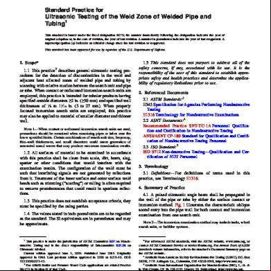
E 273 - 15 1b344z
July 2022 0More Documents from "Rostislav" 656d1g
E 2546 - 15 5q834
November 2019 35
Dao Toyota Praktika 3ea1l
December 2019 128