On The Calculation Of International Roughness Index -1501- Sayer 565cd
This document was ed by and they confirmed that they have the permission to share it. If you are author or own the copyright of this book, please report to us by using this report form. Report 3b7i
Overview 3e4r5l
& View On The Calculation Of International Roughness Index -1501- Sayer as PDF for free.
More details w3441
- Words: 7,220
- Pages: 12
TRANSPORTATION RESEARCH RECORD
1
50
I
On the Calculation of International Roughness Index from Longitudinal Road Profile Mrcrmsr W. Savnns The international loughness index (IRI) was established in 1986 by the 'World Bank and based on earlier work performed for NCHRP. IRI is calculated from a measured longitudìnal road profile by accumulating the output from a quarter'-car model and dividing by the profile length to yield a summary roughness index with units of slope. Although IRI is used widely, there is no single, short reference document that desclibes what it is and how it is calculated. Instead, the critical information is spread over several large reports. A short, self-contained reference that defines IRI is provided, along with all the information needed to compute it from longitudinal road profile measurements. The development of the IRI is reviewed, the mathematical definition is presented, an algorithm for calculating IRI is delived, the performance of the algorithm is analyzed, tested Fortran source code for computing IRI is presented, and problems with IRI (and profile measurement in general) that have emerged since 1986 are identified.
analyses included vehicle simulation with l0 alternative sets of parameters. The best correlation was obtained by using a vehicle simulation with a set of parameter values that is often called the
Golden Car. (The name is based on the concept of a golden reference instrument kept in a vault and used to calibrate other instruments.) Some researchers and s assume that the Golden Car parameters describe an average American enger car, circa 1978. This is not the case. Spring rates were selected to match the two major resonant frequencies (body and axle bounce), but damping in the Golden Car is much higher than in most cars and trucks. The high damping was chosen because the computer study showed that improved correlation with a wide variety of response-type
it
systems.
The internationai roughness index (IRI) evolved over many years, in three stages: 1. Quarter-car simulation on high-speed profilers. Routine analysis of road profiles began shortly aftel the General Motors (GM) profilometer was developed in the late 1960s by Spangler and Kelley (1). Like high-speed profilers today, it could measure true profile over a lange of wavelengths affecting vehicle vibrations. One of the first research applications for this type of system combined measured load profiles with a quarter-car computer model that replicated the Bureau of Public Roads (BPR) Roughometer, a onewheeled trailer with a road meter (2,3). GM licensed K.J. Law, Inc. to market the device commercially and continue its development. A commercial version wâs soon available that included a quafter-car analysis to summarize roughness of the measured profiles. s of early K.J. Law profilometers could choose between two quarter-car data sets: one for the BPR Roughometer and one for a 1968 Chevrolet Impala (4). 2. NCHRP research and the Golden Car. In the late 1970s, NCHRP sponsored a study of response-type road roughness measuring systems such as the BPR Roughometer and vehicles equipped with Mays ride meters. The results were published in NCHRP Report 228 (5). An objective of the study was to develop calibration methods for the response-type systems. The researchers, Gillespie and Sayers, concluded that the only valid method was caiíbration b¡- cotelation against a defined roughness index. Considerable research was performed using simulations and experitnents to compare alternative reference roughness indexes. The candidate
University
of Michigan Transportation Research Institute, 2901
Road, Ann Arbor, Mich. 48109.
Baxter
The NCHRP study provided a standard quarter-car model, and s of K.J. Law profilometels soon had access to an analysis called Mays simulation, which used the Golden Car data set. 3. World Bank development of IRI. In 1982 the World Bank initiated a correlation experiment in Brazil called the International Road Roughness Experiment (IRRE) to establish comelation and a calibration standard for roughness measurements (ó). In processing the data, it became clear that nearly all roughness-measuring instruments in use throughout the world were capable of producing measures on the same scale, if that scale had been selected suitably. Accordingly, an objective was added to the research program: develop the IRL
The main criteria in deg the IRI were that it be relevant, transportable, and stable with time. To ensure úansportability, it had
to be
measurable
with a wide range of equipment, including
response-type systems. To be stable with time, it had to be defined as a mathematical transform of a measured prof,le. Many roughness definitions were applied to the large amount of test data obtained in the IRRE. The Golden Car simulation from the NCHRP project was one of the candidate references considered, under the condition that a standard simulation speed would be needed to use
it for the IRL
After processing the IRRE data, the best conelations between a profìle index and the response-type systems were found with two vehicle simulations based on the Golden Car parameters: a quarter-car and a half-car. Both gave essentially the same level of correlation. The quarter-car was selected for the IRI because it could be used with all proflling methods that were in use at that time. The consensus of the researchers and participants is that the standard speed should be 80 km/hr (49.7 mph) because at that simulated speed, the IRI is sensitive to the same profile wavelengths that cause vehicle vibrations in normal highway use. The research findings were highly encouraging and led the World Bank to publish guidelines for conducting and calibrating rough-
TRANSPORTATION RESEARCH RECORD
2
ness measurements. The researchers (Sayers, Gillespie, Queiroz,
and Paterson) prepared instructions for using various types of equipment to measure IRI (7). The guidelines also include computer code for calculating IRI from profile. A companion report (ó) described the IRRE, using many analytical comparisons of algorithms and some sensitivity analyses. In 1990 FHWA required the IRI as the standard reference for reporting roughness in the Highway Performance Monitoring System (HPMS) (8).
OBJECTIVES OF PAPER The main objective of this paper is to provide a self-contained description of IRI, including its definition and an algorithm for its calculation. Well-tested Fortran source code for computing IRI is
provided for the benefit of those persons developing software to ar'alyze profile measurements. Previously unpublished background theory is provided about how the algorithm works, in an attempt to dispel some errors and misconceptions about IRI that have appeared in the past decade. The paper also describes some unresolved issues that have come to light after years of measuring IRI with a variety of profiling equipment and methods.
DEFINITION OF IRI The following points fully define the IRI concept; implications of these points are discussed later:
1. IRI is computed from a single longitudinal proflle. The sample interval should be no larger than 300 mm for accurate calculations. The required resolution depends on the roughness level, with flner resolution being needed for smooth roads. A resolution of 0.5 mm is suitable for alì conditions. 2. The profile is assumed to have a constant slope between sampled elevation points. 3. The prof,le is smoothed with a moving average whose base length is 250 mm. 4. The smoothed profile is filtered using a quarter-c¿ìr simulation, with specific parameter values (Golden Car), at a simulated speed of 80 km/hr (49.7 mph). 5. The simulated suspension motion is linearly accumulated and divided by the length of the profile to yield IRI. Thus, IRI has units of slope, such as inches per mile or meters per kilometer.
1
50 1
labor-intensive methods such as rod and level or DipStick, the cost of measuring two profiles is twice that of measuring one; and (c) in the research programs mentioned earlier, the coreiation between IRI and HRI was so high that the two were statistically interchangeable.
Digital Sampling Proflle analysis is nearly always performed numerically with a digital computer. The profile is sampled to obtain a sequence of elevation numbers, where each number corresponds to a different location along the profile. The longitudinal separation between samples is a constant, A, which depends on the type of equipment used to obtain the profile and possibly settings made by the operator. Filters such as the IRI quarter car are deflned for a continuous proflle, which means that there is an underlying assumption about what the profile does between samples. Figure 1 shows several possible methods for interyolating between sampled values:
I. Zerc slope between points implies a discontinuity in elevation at each sample location, 2. Linear interpolation between points implies a constant slope, and 3. Quadratic interpolation maintains continuity in both elevation and slope through the sample values. A computer study was done in the preparation for the IRRE to determine which of the three interpolation methods gave ihe best accuracy for various values of A. All three methods give the same IRI values when A is very small, on the order of 50 mm (2 in.) or smaller. However, for larger A-values, results calculated using Option I were too high, results calculated with Option 3 were too low, and results calculated with Option 2 were reasonably accurate. For larger sample intervals, the results were too low even with Option 2. These results lead to the assumption, built into the IRI, that the profile between sampled measures is a straight line connecting the points. Limits were set on the sample interval: 300 mm for accu¡ate measures and 600 mm for less accurate measures with some bias.
IRI Filter The IRI includes two distinct filters: a moving average and
a
quarter-car model.
IRI Input Number of Profiles
Moving Average
The IRI is defrned as a property of a single wheel-track profile. For systems that measure several profiles simultaneously, it is calculated independently for each.
The moving average was included for two reasons: (a) to simulate the enveloping behavior of pneumatic tires on highway vehicles,
An alternative analysis is sometimes done when two prof,les are measu¡ed at the same time. The proflles are averaged, point by point, and then processed using the IRI algorithm. This form of analysis is called a half-car simulation, and it is not the same as IRI. Similarities and differences between the half-car roughness index (HRI) and IRI are discussed elsewhere (9). IRI was defined fol a single wheel-track profile because (a) many proûler instruments can measure only one profile at a time; (å) for
rul khbl'tllru FIGURE I Methods for interpolating between profrle samples: left, zero slope-hold previous value; middle, constant slopelinear interpol ation; right, continuous slope-quadratic interpolation.
3
Sayers
and (å) to reduce the sensitivity of the IRI algorithm to the sample interval, Â. For a profile that has been sampled at A, a moving average smoothing filter is defined by the summation
tn¡,
I ¡+k I h^(t): : ) h,l.t) 'k-.
'"
ft
:
: : k,: ¡??r : c.
suspension damping rate suspension spring rate fire spring rate
k"
sprung mass (portion of vehicle body mass ed by one wheel) unsprung mass (mass of wheel, tire, and half of axle/suspension)
:
(1)
'): '
(2)
max[1, nin(L'lÂ)]
To simplify the equations, the parameters are normalized by the sprung mass, m".The following values for the normalized parameters define The Golden Car data seT'.
where
: /ro" : max : nint : 16 : /zo
kt
smoothed profile height,
maximum of two arguments, nearest integer, and moving average base length, 250 mm.
For example,
: c"lm": 6.0 : þ,/¡n": 653 kr: þ"1s, : 63.3 lL: m,,/m" - 0.15 c
profile height,
if the sample interval is A :
150 mm (6 in.), the ratio
(l¡lÂ) is 1.67, which is rounded to 2. The number 2 is larger than 1, so k is set to 2.
Digital profilometers made by K.J. Law, Inc. have often been used in American research programs. The data acquisition software
in the digital K.J. Law systems has always included a movìng average of 300 mm. The difference between a 250-mm and 300-mm moving average on IRI is negligible. Thus, the moving average part of the IRI results in a high degree of compatibility with Law profilometers. However, it is important that this averaging not be performed a second time when IRI is calculated from profiles measured
The quarter-car model is described by four first-order ordinary differential equations that can be written in matrix form:
i:Ax+Bhp"
Ø)
where the x, A, and B arrays are defrned as follows:
x:
lz",
1000 kz -k2 -c 0010 c_ þ ppl-ttr _kt*k,
A:
with Law systems. (Read the comments in the IRI code presented later in Figure 6.).
B Quarter Car
(3)
:
c
(s)
I0, 0,0,k/¡t"lr
where
: : 2,, : x:
Figure 2 shows the quarter-câr model in the IRI. It includes the
smoothed profile elevation, height (vertical coordinate) of sprung mass, height (vertical coordinate) ofunsprung mass, and affay of state variables (variables that, together, completely describe state of simulated system).
år.
major dynamic effects that determine how roughness causes vibrations in a road vehicle. The masses, springs, and dampers are defined by the following parameters:
z"
i). Time is related to longitudinal distânce by the simulated speed of the vehicle Time derivatives are indicated with a dot (e.g.,
t: Forward Speed: V = 80 km/h z
l-r* 1
(6)
x/V
where x is longitudinal distance and y is the simulated forward speed. Vis defined as 80 km/hr (49.7 mph) for the IRI. The units of V should be length/second, where the units of length match those of x (e.g., V : 22.222 mlsec : 72.90'155 ftlsec).
IRI Accumulator The IRI is an accumulation of the simulated motion between the sprung and unsprung masses in the quarter-câr model, normalized by the length L, of the profile:
L, FIGURE
2
= 250 mm
Quarter-car model.
rRr:
l I T.
lz"
*
(1) ;,,10,
TRANSPORTATION RESEARCH RECORD
4
I
501
The vehicle response variables oscillate about 0 and have 0 as an average value. The absolute value in equation 7 is needed to obtain a non-zero averâge. Another method that might have been selected, but was not, is root mean square (RMS). RMS averaging is less convenient to use because it is nonlinear with respect to absolute amplitude, whereas equation 7 is linear. For example, if the IRI of a 0.5-
of ordinary dffirential equations." Equations in this form can be solved by several methods. Thus, the IRI can be calculated by more than one method. In this section, two methods are presented and
mi section is 100 in/mi, and the IRI for the next 0.5-mi section is 200 in./mi, the IRI for the entire mile is the simple linear average:
Euler Integration (Not Recommended)
150 in./mi. In contrast, the RMS average would be 158. Another reason for using linear averaging was to match the behavior of existing road meters.
The most common way to solve ordinary differential equations is by numerical integration. There are many numerical integration algorithms (10). The simplest, known as Euler integration, applies the approximation
Initialization
X¡=X¡-r
To solve differential equations such as equation 4, one must know
where dr is a small time interval proportional to the sample interval
or estimate the values of the state variables at the starting time. The rcsponse obtained over a profile includes a response of the transition from the initial values to the profile-induced response. The effect of the initìalization diminishes as the simulated car covers more of the profile. At the IRI simulation speed of 80 km/hr, the initialization influences the quarter-car response for about 20 m. The most accurate way to deal with the initialization is to measure the profrle for 20 m or so before the site and start the simulation there. Then, at the staft ofthe test site, begin the IRI accumulation (equa-
tion 7). A computer study was made to find an initialization method that minimizes errors in the first 20 m (ó). It led to the recommendations that, initially, z, and 7,, should be set to match the height of the first profile point and that 2. and 2, should be set to match the average change in profile height per second, at the simulation speed of 80 km/hr, over the first 1 1 m ofprofile.
compared.
+ dtii
(8)
I
dt: NV
(9)
IRI can be calculated using the Euler approximation if the interval between profile samples is sufficiently small; Figure 3 addresses the question of what is sufficiently smail? The figure, which shows the output of the algorithm as a function of wavenumber (wavenum1/wavelength), indicates that the algorithm is in enor even ber for sample intervals as small as 10 mm. As the intervals grow to 100 mm (4 in.), the effors become worse. If one is committed to using Euler integration, it is recommended to generate more profile points by linear interpolation to obtain a sample interval of 10 mm or less. The need for a very small interval requires the computer program to perform the calculations many times between the profile measure-
:
ments, seriously reducing the overall calculation speed.
Recommended Algorithm
IRIALGORTTHM Theory Equations I through 7 define the IRI. The quarter-cardynamics and the initialization method together make up a type of calculation whose generic name is "the initial value problem," or "integration
For a set of linear equations such as equation 4, the total responsè at point i is the sum of thefree response (no input) of the system to
A=10mm ^=0 A=25mm Â=50mm À=100m
.-l
_t l0l Wavenumber (cycles/m) FIGURE
3
Euler integration response plots.
5
Sayers
its state at a previous point i- I , plus the forced response to an input over the interval between points i- I and i. In the case that the input is a constant, the closed-form solution is known: x¡
:
eANv
x¡ t
| (e^Nv
+
^
(10)
-l)ßu
Although the state variables in equation 13 are different from those first presented in equation 5, they are also suitable for defining IRI. Specifically, equation 7 can be transformed to
I Fl',,, -',,,1 1n
rRr:
(14)
n i=:
where
: I : ø: ¿
of natural logarithms, 4 identity matrix, and input that is constant over interval base
4
The smoothed profile slope, based on a 250-mm interval, is computed with the simple difference equation
x
i
-
1
to i.
The term eAAlv is a 4 x 4 state transítion matrix that defines the free response as a linear combination of the four variables in x at point i - 1, and term L-t (e^Ltv - I) B is a four-element partial response alTay that defines the forced response as a linear function of ø. The exponential of a matrix can be calculated several ways, one of which is a Taylor series expansion:
e^Nv-
.M. A(A/\4i
(11)
I+ 4;l )
h
"Ps.i
p,¡+ t,
-
h
p,i
(1s)
kL
where fr was defined in equation 2.
The IRI deflnition of equation 14 is generalized in the computer code as
IRI
: 1É1"'l
(16)
i:i
-
where N is a number large enough that the elements of the state transition matrix are correct to within the precision of the computer. Equation 10 is exact to the extent that the input ø is actually con1 to i. Recall that research of stant over the interval from point i different interpolation methods showed that the best approximation of the sampled profile to a continuous one is that the profile slope is constant between samples. This means that to obtain the best accuracy, the assumed constant input a in equation 10 should be proñle slope. Then, equation 10 is the solution for the differential equations
where matrix C is defined as:
Ç=[10-10]
-
*=Ax*Bsp,
x
:
To initialize the algorithm, the elements of the x array for I
:1
are set as
x1
:l(hr.t¿t- hp.)|L.,0, (ho.t¿r-hpìlL.' 0l
where
l,
(18)
is l1 m.
(12)
is smoothed profile slope. However, replacing frr" with s^ implies that the array x is redefined as where
(17)
Performance
so"
[s,, s,, s,,,
s,,]t
(13)
where s" and s,, are fìltered slope variables associated with the sprung and unsprung masses.
Figure 4 shows the response of the recommended algorithm for several sample intervals. The plots show the state transition method to be much less sensitive to changes in sample interval than the Euler integration method. (Note that the intervals used in Figure 4 are
much larger than those shown for the Euler integration method in Figure 3.)
Quarter-car response (dimensionless)
rÁ=0 :Á=50mm ì^ = 150 mm
i = 300 mm
Â=600mm
0.5 :
0r
l0-l
l0-2
i00
Wavenumber (cYcles/m)
FIGURE
4
Response of recommended
algorithm.
-l 10r
TRANSPORTATION RESEARCH RECORD 1 50
Ratio:
1
Computeü!l True lRl
State Transition :
:-ìr
100 mm Sample lnterval
FIGURE
5
10m
Error in IRI due to sample interval for two algorithms,
Figure 5 shows theoretical relations between sample interval and roughness over wavenumber. It shows that noticeable eûor exists when the Euler integration is used, even for an interval as small as A : 10 mm. As the step grows to 100 mm, the error is about 1 8 percent. In conÍast, the state transition method has negligible eror until the sample interval reaches 200 mm. The error ¡emains less than 2 percent at A : 300 mm, ing the original reqr"rirement of a 300-mm interval (or smaller) for accurate IRI calculations. However, the original specifrcation of 600 mm for Class 2 measures is associated with a theoretical bias of more than 10 percent, which is probabiy too much error for most applications. The exact relationship between sample interval and IRI is specific to a particular profile. The plot in Figure 5 applies to proflles with a typical distribution. A road with proportionally more long-wavelength roughness could be measured with less effor than indicated, whereas higher enors would be obtained for a road with proportionally more shoft-wavelength roughness.
IRI for a road with.a typical distribution of
quafter-car models, Butterworth fllters, etc.). Subroutine SETABC (Figure 7) sets up the A, B, and C matrices based on quarter-car parameters. (See equations 5 and 17.) Subroutine SETSTM (Figure 8) computes the state transition (ST) and partiai response (PR) matrices, given the A and B matrices and a time step DT. It requires a routine INVERT for inverting a square matrix. The code for INVERT is not shown to conserve space, given that suitable matrix algorithms are readily available (10). Subroutine STFILT (Figure 9) filters the profile using the state transition method. The listed code was written for generality and clarity rather than being optirnized for efficiency. The algorithm itself is fast enough
that coding efficiency
is
usually not an issue with modern
microcomputers. Fully operational profile analysis software is available at no cost from the University of Michigan Transportation Institute (UMTRÐ including the source files shown in the listings. the author for information on acquiring the software and source code.
PROFILE MEASUREMENT Computer Listings Figures 6-9 show tested computer routines for calculating IRI, programmed in the Fortran language. The algorithms are simple enough that translation to other languages (e.g., C) should not be too
difficult. Subroutine IRI (Figure 6) should be applied to a profile represented as a one-dimensional array of floating-point numbers. In addition to computing a summary IRI value, the subroutine replaces the original profile (å,,,J with a proflle filtered with the IRI moving average and Golden Car. This routine contains all details that are highly specific to the IRI, such as (ø) the specific numerical values of the Golden Car parameters, (å) the simultaneous conversion of profile elevation to profrle slope and smoothing via equation I 5, (c) the initialization of the filter with the average profile slope over the ûrst 11 m, and (d) the accumulation of absolute frltered slope to obtain IRI. The subroutines in Figures 7-9 are required by the IRI routine; they can also be used for profile analysis applications other than IRI, for filters represented by four differential equations (e.g., other
The IRI definition describes a method for computing a roughness index for a single longitudinal profile of arbitrary length. Its accuracy and relevance are limited by the quality of the profile measurement, which depends on (a) the design and quality of the equipment, and (å) the methodology and care used to make the measurement. Following are some ways that profile measurement affects IRI.
Location and Width of Profile Recall that IRI is defined as a property of single longitudinal profile, measured along a single line down the road. s often want an overall IRI for a traveled lane. This raises two questions: How many profiles should be taken for a traveled lane? and At what lateral position(s) should the longitudinal prof,le(s) be measured? The IRI definition does not address this issue, although the recommendation is that the profiles should be measured in two Íaveled wheel tracks, with the IRI values for each being averaged to obtain a sum-
._
===
================== ======= = == ---SUBROUTTNE TRI(PROF, NSAMP, DX, BASE, UNTTSC, AVEIRT)
C Filter
a longitudinal road profi]e and calculate IRI '
inputf an array of profile height values. on output, an array of filt.ered profile values. C <-> NSAMP fNTEGER Number of data samples in array PROF. The filtered profile has fewer points Lhan the origrínal ' C Distance step between profile points (m). REAL C --> DX Distance covered by moving average (n). C --> BASE REAL Use 0.250 for unfiltered profile input, and 0.0 C for pre-smoothed prof iles (e.9. K.,f . Law data) . C of two scale facLors: (1) meters per unit Product C --> UNITSC REAL of profile height, and (2) IRI units of slope. C Ex: height is inches, slope will be in/mi. C UNITSC = (.0254 m/in)*(63360 inlmi) = 1069.34 C The average IRI for the entíre profile' <-REAL AVEIRI C C <-> PROF REAL
C
On
INTEGER I, TLl., IBASE, J, NSAMP AMAT, AVEIRI, BASE, BMAT, CMAT, DX, PR, PROF' SFPT, ST
REAL REAL
DTMENSTON
&
UNITSC, AMAT(4,
V, XTN 4), BMAT(4), CMAT(4), PR(4),
PROF(NSÄMP) ,
sr(4,4), XrN(4)
C Set parameters and arraYs. CALL SETABC(653.0, 63.3, 6.0, 0.15, .AMAT, BMAT, CMAT) CALL SETSTM (DX/ (80. /3 .6) , AMAT, BMAT, ST, PR) IBASE = MAX(INT(BASE/DX + 0.5)' 1) SFP] = IINTTSC/ (DX*IBASE) C IniLialize simulation variables based on profile start. Il-1 = MIN(TNT(11-./DX + .5) + 1, NSAMP) XIN(1) = UNfTSC* (PROF(I11) - PRoF (t)l / (Dx*I1-1) xrN(2) = 0.0 xrN(3) = xrN(j-) xrN(4) = 0.0 C ConverL to averaged slope profile, wíth IRI units. NSAMP=NSAMP-TBASE DO 10 I = 1' NSAMP 10 PROF(I) = SFPI*(PROF(I
+ IBASE) -
C Filter profile.
PROF(I))
CALL STFILT(PROF, NSAMP, ST, PR, CMAT, XIN)
C Compute IRI from filtered profile. AVEIRI = 0.0 DO 20 I = 1, NSAMP 20 AVEIRI = AVEIRI + ABS(PROF(I)) AVETRI = AVETRI/NSAMP RETURN END
FIGURE
6
Fortran code to calculate IRI from profile.
TRANSPORTATION RESEARCH RECORD 1 50]
^-- ---- --
- - -- ---= = ==== ===== =========== === = == === ===== ========= ====-== SUBROUTINE SETABC(KI, K2, C, MU, AMÀT, BMAT, CMAT)
====
u-------^--------
C Set the A, B and C matrices for the a t/4 car model' C
K1 REAL c --> K2 REAL REAL C --> C C --> MU REAL C <-- AMÀT REAL C <-- BMÀT REAL C <-- CMAT REAL C -->
KtlMs = normalized Ks/Ms = normalized Ks/Ms = normal-ized Ks/Ms = norftalized The 4x4 A matrix. The 4x1 B matrix. The 4x1 C matrix-
tire spring rate (I/s/s) suspension spring rate (1/s/s) suspension damper rate (1/s)
unsprung mass (-)
TNTEGER T., ,J À¡44T, BMAT, CMAT, K1 , R2, C, MU REAL DIMENSION AMAT(4, 4\ , BMAT(4), CMAT(4) C Set default for all matrix elements to zero' DO10J=L,4 BMÀT(J) = 0 cMÀT(J) = 0 DO101=L,4 AMAT(I, J) = 0 1-0 C Put I/4 car model parameters into the A Matrix' AMAT(1, 2) = 1. AMAT(3, 4\ _ T. ÀMAT(2, 1) - -K2 AMAT(2' 2\ = -C AMAT(2, 3) = R2 AMAT(2, 4) = C AMAT(4, 1) - K2/YF¿ AMAT(4, 2) = C/MU AMAT(4, 3) = -(K1 + K2) /t{u AMAT(4, 4\ = -CIMU C Set the B maLrix for road inpuL through tire spring' BMAT(4) = K1IMU C Set the C matrj.x to use suspension motion as output ' CMAT(1) - -1 CMAT(3) = 1 RETURN END
FIGURE
7
Code to set model matrices.
mary IRI for the lane. Obviously, agreement between measures obtained for a given road by different s is limited unless they choose the same profile locations. A related issue is the width of the profile. Laser-based systems measure a proûle that coffesponds to a line several millimeters wide. K.J. Law optical systems measure a line that is about 6 in. wide. DipStick measurements detect the profrle under pads that
not or not
have a fixed diameter. To this author's knowledge, research has been done to the determine the effect of profile width on the IRI any other roughness statistic. (And, by the way, the IRI does
specify a profile
width.)
Length of Profile The test sites used in developing IRI a1l had a length of 320 m (about 0.2 mi). In more recent resea¡ch studies, 0.1-mi sites are common. Theoretically, IRI can be computed for any length of profile. However, s must realize that the variation in IRI down the road depends on the length over which it is accumulated. When IRI is summarized for l-mi sections in routine survey work, the highest values (roughest sections) are not as high as when IRI is summa-
rized for 0.1-mi sections. Short distances (e.g., 50 ft) isolate local effects such as faults and produce very high IRI values (11).
r_========
SUBROUTINE SETSTM(DT, L======== ^______-_ C Compute ST and PR c
c --> c--> C-_>
DT A
C <-_
PR
REAL REAL REAL REAL REAL
B
c <-- sr
arrays. This requires
I, ]TER, J, MORE
= I' 4 1 = )-, A1 (r, ,J) sr (r,
20 C
c
J) -
(J, J) = ST(J, J) =
AL
K
A, A1, A2, B, DT, PR, ST, TEMP A(4, 41 , Ar(4, 4), A2(4, 4l , B(4), PR(4), ST(4, 4), TEMP (4, 4 )
DO 20 J DO 10
l-0
for matrix inversion.
4x4 sLate transition matrix. 4x1 partial response vector.
TNTEGER
DTMENSION
INVERT
Time step (sec) The 4x4 A matrixThe 4x1 B matrix.
LOGICAL REAL
A, B, ST, PR)
4 0 0
1. L.
Calculate the state transition matrix ST = exP(dt*A) with a îay1or series. Al- is the previous Eerm in the series, A2 is Lhe next one. ITER = 0 30 rTER - rTER + 1 MORE = .FALSEDO40J=L,4 DO40 l=1,4 A2(r, J) = 0 DO40K=1,4 A2(I, J) = A2(I, J) + A1 (r, K) * A(K, J) 40 50 J = l, 4 DO50 I=L,4 A1(I, J) _ A2(I, J)T'DT/TTER IF (ST(I, J) + A1(1, J) .NE. ST(r, J)) ST(1, J) = ST(f, J) + À1 (I, ,J)
DO
50
IF
MORE
=
.TRUE.
(MORE) GO TO 30
C CafculaLe particular response matrix: PR = A*'(-1* (ST-I)*B CALL INVERT (4, 4) DO60 I=L,4 PR(r) - 0.0 DO60K=I,4 PR(r) = PR(I) - A (r, K) *B (K) 60 DO 90 J = I, 4 DO 70 I = L, 4 TEMP(J, l) = 0.0 DO 70 K = 1, 4 TEMP (J, I) = TEMP(J, I) + A(J, K)*ST(K, I) 70 DO80K-I,4 PR(J) = PR(J) + TEMP (J, K) *B (K) 80 9O CONTTNUE RETURN END FIGURE
I
Code to set stâte transition matrix.
TRANSPORTATION RESEARCH RECORD
1
50]
4----
SUBROUTTNE STFILT(PROF, NSÀMP,
ST, PR, C, XIN)
C Filter profile using matrices sT, PR, and c C
C C C C C
<-> --> --> --> --> -->
PROF REAL
C.
Input profile. Replaced by the output. of data values in array PROF. 4x4 state transition matrix. 4x1 parLial- response vector. 4x1 output definition vecLor. Initial values of filter variables.
NSAMP fNTEGER Number
ST PR C XIN
REAL REAL REAL REAL
INTEGER I, J, K, NSAMP C, PR, PROF, ST, X, XIN, XN DTMENSTON C(4), PR(4), PROF(NSAMP), ST(4, 4), X(4\, XrN(4), XN(4)
REAL
C Initialize simulation variables. DO10L=I,4 1-0 x(I) = xIN(I) C Filter profile using the state transition algorithm. DO 40 I = 1, NSAMP DO 20 J = L, 4 XN(J) = PR(J)*PROF(I) DO 20 K = 1, 4 20 XN(J) = XN(J) + X(K)*ST(J, K) DO 30 J = 1, 4 30 X(J) = XN(J) PROF(1) = x(1)*c(1) + X(2)*C(2) + x(3)*C(3) + X(4)*C(4) 40 CONT]NUE RETURN END
FIGURE
9
Code to filter profile.
It is essential that planners and engineers using IRI understand this fundamental relationship between roughness variation along the road and the length ofthe road over which the roughness is averaged. Local uses of IRI for pavement management and evaluation of newly constructed pavements should specify a standard length, especially when IRI is used to identify maximum roughness.
Cracks Profilers with laser sensors can detect cracks, tar strips, patches, and other small bumps. Short events such as these appear as spikes tn the profile, which partially reduces the effect ofsuch spikes through the 250-mm moving average. However, their influence is not completely eliminated. Consequently, laser-based systems sometimes produce higher IRI measures than other systems. Bumps are highly objectionable to road s, while cracks go unnoticed. A profiler that can detect bumps should obtain a more accurate and representative IRI value than a profrler that cannot. On the other hand, a profiler that is sensitive to cracks is subject to at least two error sources. First, the extra IRI roughness due to the crack is not indicative of roughness as perceived by the traveling public. Second, the effect is not completely repeatable. Although a system might detect the same crack in repeat measures, the depth of
the crack depends on many variables, including the amount of dirt in the crack and the precise lateral location of the laser. In one , the crack might appear to be 5 mm deep; in a subsequent , it might be seen as 50 mm deep. Most prof,lers store datâ at intervals of 100 mm or more. Once the information is recorded, it is not possible to tell the difference between a crack that is several millimeters wide and a depression that is twice the sample interval (e.g., 200 mm in length). Therefore, it is usually not possible to identify cracks after- the measurement is made. The recommended solution is for developers of laser-based profilers to install real-time crack detection software. Ifenabled (for
roughness measurement), the software should hold the previous value when the laser goes into a crack. The algorithm must distinguish between bumps, which cause roughness, and cracks, which do not. Linear filtering does not distinguish between bumps and cracks and therefore is not sufficient. The problem of cracks is not unique to IRI. It exists with almost any roughness index.
Reference Profilers World Bank Report 46 defrned two classes of profiling methods that were late¡ adopted by FHWA for the HPMS data base (28). Profll-
l
I
I
1l
Sayers
if they produce IRI measures that are neither high nor low on the average. However, an individual measurement is expected to have random error. Some profilers clearly are more accurate than others, so the concept of a Class 1 measurement was introduced to define a reference that can be used to detemine the accuracy of other instruments. A Class 1 instrument must be so accurate that the random enor is negligible; its IRI measure is "the ers are considered Class 2
truth." On the basis of data available at the time of the IRRE, the level accuracy associated with Ciass 1 was set at +2 percent for 320-n (0.2-mi) test sites. Computer studies of the sensitivity of IRI to sample interval and height lesolution we¡e used to define a Class I prof,ling insÍument. The concept of classes for profrlel methods has proved popular among s and manufacturers. Folexample, ASTM recently approved a standard (not yet published) on inertial profilers that establishes four classes of profilers. However, evidence from correlation studies over the past 10 years indicates that current specifications of a Class I IRI profile measurement al'e not sufficient. Devices that on paper qualify as Class 1 do not âlways show the repeatability that was expected. In retrospect, the major problem is that the speciûcations focus on the equipment and not its use. Even with highly experienced operators, human er¡or sometimes results in an inconect profile measurement, thus an incorrect IRI. (For example, operators can start the measurement too soon or too late, or locate the instrument in the wrong lateral position.) Some limitations with the equipment are not covered by the specifìcation of sample interval and height resolution. Experience now shows that a device might have trouble with a specific road surface. A common example is that certain textured surfaces can confuse even the best noning height sensors used in high-speed profrlers. Another example is that the DipStick, which captures samples of profile height every 300 mm, can miss signifìcant roughness
of
on a surface with bumps just several inches long. Hardware specifications can qualify adevice as Class 1-capable, but, as a minimum, repeat measures are needed to qualify the mea-
sures taken on a specific site. Repeatability is better with static devices such as the DipStick. However, good repeatability does not always imply good accuracy. If the profile measurement is always started at the same point (with a tolerance of an inch or so), the IRI can be highly repeatable but incorrect if the sample interval (A) is not sufficient to capture all signiflcant roughness. Thus, for static measures, repeat measures should be made at slightly different starting locations. As experience is gained, areas emerge where differences between
instruments are not easily explained. For example, it is known that profiles of some roads change significantly with temperature. Provisions must be made to fo¡ this effect in the acquisition of
profile data for research involving Class I methods. Research is needed to refine the definition of a Class 1 measurement. As a minimum, the specification should be extended to describe a test method for using the instrument that allows the to estimate its quality (e.g., by looking at the scatter in repeated measures).
CONCLUSION When the IRI was defined in World Bank Technical Report 46, there were only about a half-dozen inertial profilometers in America. Since then profiling has become the primary means for mea-
suring road roughness in the United States. More than half the states have purchased or built profiling systems. The fedelal government maintains a fleet of profilers for calibration and research programs, and consulting companies maintain profrling systems to provide
to states and local districts that do not have their own equipment. FHWA has encouraged profiler use and has sponsored several correlation experiments. Profiler s have organized into the Road Profiler Group, which has established an annual cor¡elation experiment for several years in which s are invited to measure profiles and IRI for test sites. The profilers in use cover a wide variety of sensor types, cost, and analysis options. Limited by the speed of sound, systems with ultrasonic sensors can measure profile at intervals no closer than about 300 mm (1 ft) at highway speeds. Other systems, with laser sensors, can measure at intervals going down to a few millimeters. Some systems perform minimal profrle frltering. Others routinely smooth the data to avoid aliasing and remove long wavelengths to standardize plot appearances. Even with these differences, most profilers in use can obtain IRI measures that show reasonable agreement measures
(within 5 percent). However, recent conelation experiments show that no existing profiler can measure "true IRI" with the high accuracy one might expect of a Class I instrument (i.e., within 2 percent). Further research is needed to dete¡mine the reasons that consistent measures
of roughness are not obtained. Two possible sources of discrepancy are practice and changes in road profile due to temperature and environmental effects.
ACKNOWLEDGMENTS Steve Karamihas of UMTRI assisted with the preparation of this paper and provided the theoretical response plots. The preparation of this paper was funded by FHWA. Elson Spangler of Surface Dynamics and John Darlington of the Michigan Depaltment of Transportation first applied quarter-car simulation to measure road profiles in the early 1970s. Spangler also served on the scientific committee for the work described in NCHRP Report 228 and was an eariy advocate of a Golden Car mathematical model. Rudy Hegmon of FHWA also participated in the NCHRP work and has long been an advocate of proflle-based measures of road roughness. Hegmon has led FHWA's involvement in profiler technology since the late 1970s; he initiated the development of FHV/A's PRORUT system. Thomas Giilespie of UMTRI was the principal investigator for the NCHRP project, technical director of the World Bank Research progrâm in which IRI was developed, and coauthor of the IRI specifications. Cesar Queiroz (now with the World Bank) was the overall director of the World Bank project, which was run by the Brazilian Road Research Institute (IPR/DNER) and the Brazilian Transportation Planning Agency (GEIPOT). William Paterson of the World Bank was an early advocate of the development of an IRI and a coauthor of the IRI specifrcations. The late Per Fossberg of the World Bank contributed to the final stages ofthe IRI development and the publication of World Bank Technical Reports 45 and 46. The person most responsible for the existence of the IRI is Clell Harral of the World Bank. Harral conceived the idea of the IRI and arranged for the participation ofthe various technical personnel who developed the specifications, tested them, and wrote the guidelines for applying them.
TRANSPORTATION RESEARCH RECORD I 501
t2
7.
REFERENCES
3. 4. 5. 6.
Evaluating Road Surface Roughness. Public Roads, Feb. 1941. Darlington, J.R. Evaluation and Application Study of the General Motors Corporation Rapid Travel Profilomefer. Research Report R-731. Michigan Department of State Highways, Lansing, Oct. 1970. Burchett, J. L., et al. Surface Dynamics Profilometer and Quarter-Car Simulator: De scription, Evaluation, and Adaptation. Research Report 465. Kentucky Department of Transportation, Frantfort, 1977. Gillespie, T. D., M. W. Sayers, and L. Segel. NCIIRP.R eport 228: CaIibration of Response-Type Road Roughness Measuring Systems. TRB, National Research Council, Washington, D.C., Dec. 1980. Sayers, M. W., T. D. Gillespie and C. Queiroz. International Experíment to Estctblish Correlations and Standard Calibration Methods for Road Roughness Measurementl World Bank Technical Paper 45. World Bank, Washington, D.C., 1986.
for the
Conduct and Calibration of Road Roughness Measurements. World Bank Technical Paper 46. World Bank, Washington, D.C., 1986. 8. Highway Performance Monitoring System, Field Manual, Appendix J. Order M 5600.14. FHWA, U.S. Depaftment of Transportation, April
l.
Spangler, E. 8., and W. J. Kelly. GMR Road Profilometer, a Methodfor Measuring Road Profrle. Research Publication GMR-452. General Motors Corp., Wanen, Mich. Dec. 1964. 2. Buchanan, J.,{., and A. L. Catudal. Standardizable Equipment for
Sayers, M. W., T. D. Gillespie, and W. D. Paterson. Guidelines
1990. Sayers, M. W. Two Quarter-Car Models for Defining Road Roughness: IRI and HRI. InTransportation Research Record 1215, TRB, National Research Council, Washington, D.C., 1989, pp. 165-172. 10. Press, W., et al. Numerical Recipes: The Art of Scíentffic Computing. Cambridge University Press, England, 1986. [1. Sayers, M. W. Profiles of Roughness. ln Transportation Research
9.
Record 1260, TRB, National Research Council, Washington, D.C., 1990, pp. 106-1 1 1.
Publication P
of this paper
rop e rtie s-Vehic le Inte raction.
sponsored
by
Committee
on
Surface
1
50
I
On the Calculation of International Roughness Index from Longitudinal Road Profile Mrcrmsr W. Savnns The international loughness index (IRI) was established in 1986 by the 'World Bank and based on earlier work performed for NCHRP. IRI is calculated from a measured longitudìnal road profile by accumulating the output from a quarter'-car model and dividing by the profile length to yield a summary roughness index with units of slope. Although IRI is used widely, there is no single, short reference document that desclibes what it is and how it is calculated. Instead, the critical information is spread over several large reports. A short, self-contained reference that defines IRI is provided, along with all the information needed to compute it from longitudinal road profile measurements. The development of the IRI is reviewed, the mathematical definition is presented, an algorithm for calculating IRI is delived, the performance of the algorithm is analyzed, tested Fortran source code for computing IRI is presented, and problems with IRI (and profile measurement in general) that have emerged since 1986 are identified.
analyses included vehicle simulation with l0 alternative sets of parameters. The best correlation was obtained by using a vehicle simulation with a set of parameter values that is often called the
Golden Car. (The name is based on the concept of a golden reference instrument kept in a vault and used to calibrate other instruments.) Some researchers and s assume that the Golden Car parameters describe an average American enger car, circa 1978. This is not the case. Spring rates were selected to match the two major resonant frequencies (body and axle bounce), but damping in the Golden Car is much higher than in most cars and trucks. The high damping was chosen because the computer study showed that improved correlation with a wide variety of response-type
it
systems.
The internationai roughness index (IRI) evolved over many years, in three stages: 1. Quarter-car simulation on high-speed profilers. Routine analysis of road profiles began shortly aftel the General Motors (GM) profilometer was developed in the late 1960s by Spangler and Kelley (1). Like high-speed profilers today, it could measure true profile over a lange of wavelengths affecting vehicle vibrations. One of the first research applications for this type of system combined measured load profiles with a quarter-car computer model that replicated the Bureau of Public Roads (BPR) Roughometer, a onewheeled trailer with a road meter (2,3). GM licensed K.J. Law, Inc. to market the device commercially and continue its development. A commercial version wâs soon available that included a quafter-car analysis to summarize roughness of the measured profiles. s of early K.J. Law profilometers could choose between two quarter-car data sets: one for the BPR Roughometer and one for a 1968 Chevrolet Impala (4). 2. NCHRP research and the Golden Car. In the late 1970s, NCHRP sponsored a study of response-type road roughness measuring systems such as the BPR Roughometer and vehicles equipped with Mays ride meters. The results were published in NCHRP Report 228 (5). An objective of the study was to develop calibration methods for the response-type systems. The researchers, Gillespie and Sayers, concluded that the only valid method was caiíbration b¡- cotelation against a defined roughness index. Considerable research was performed using simulations and experitnents to compare alternative reference roughness indexes. The candidate
University
of Michigan Transportation Research Institute, 2901
Road, Ann Arbor, Mich. 48109.
Baxter
The NCHRP study provided a standard quarter-car model, and s of K.J. Law profilometels soon had access to an analysis called Mays simulation, which used the Golden Car data set. 3. World Bank development of IRI. In 1982 the World Bank initiated a correlation experiment in Brazil called the International Road Roughness Experiment (IRRE) to establish comelation and a calibration standard for roughness measurements (ó). In processing the data, it became clear that nearly all roughness-measuring instruments in use throughout the world were capable of producing measures on the same scale, if that scale had been selected suitably. Accordingly, an objective was added to the research program: develop the IRL
The main criteria in deg the IRI were that it be relevant, transportable, and stable with time. To ensure úansportability, it had
to be
measurable
with a wide range of equipment, including
response-type systems. To be stable with time, it had to be defined as a mathematical transform of a measured prof,le. Many roughness definitions were applied to the large amount of test data obtained in the IRRE. The Golden Car simulation from the NCHRP project was one of the candidate references considered, under the condition that a standard simulation speed would be needed to use
it for the IRL
After processing the IRRE data, the best conelations between a profìle index and the response-type systems were found with two vehicle simulations based on the Golden Car parameters: a quarter-car and a half-car. Both gave essentially the same level of correlation. The quarter-car was selected for the IRI because it could be used with all proflling methods that were in use at that time. The consensus of the researchers and participants is that the standard speed should be 80 km/hr (49.7 mph) because at that simulated speed, the IRI is sensitive to the same profile wavelengths that cause vehicle vibrations in normal highway use. The research findings were highly encouraging and led the World Bank to publish guidelines for conducting and calibrating rough-
TRANSPORTATION RESEARCH RECORD
2
ness measurements. The researchers (Sayers, Gillespie, Queiroz,
and Paterson) prepared instructions for using various types of equipment to measure IRI (7). The guidelines also include computer code for calculating IRI from profile. A companion report (ó) described the IRRE, using many analytical comparisons of algorithms and some sensitivity analyses. In 1990 FHWA required the IRI as the standard reference for reporting roughness in the Highway Performance Monitoring System (HPMS) (8).
OBJECTIVES OF PAPER The main objective of this paper is to provide a self-contained description of IRI, including its definition and an algorithm for its calculation. Well-tested Fortran source code for computing IRI is
provided for the benefit of those persons developing software to ar'alyze profile measurements. Previously unpublished background theory is provided about how the algorithm works, in an attempt to dispel some errors and misconceptions about IRI that have appeared in the past decade. The paper also describes some unresolved issues that have come to light after years of measuring IRI with a variety of profiling equipment and methods.
DEFINITION OF IRI The following points fully define the IRI concept; implications of these points are discussed later:
1. IRI is computed from a single longitudinal proflle. The sample interval should be no larger than 300 mm for accurate calculations. The required resolution depends on the roughness level, with flner resolution being needed for smooth roads. A resolution of 0.5 mm is suitable for alì conditions. 2. The profile is assumed to have a constant slope between sampled elevation points. 3. The prof,le is smoothed with a moving average whose base length is 250 mm. 4. The smoothed profile is filtered using a quarter-c¿ìr simulation, with specific parameter values (Golden Car), at a simulated speed of 80 km/hr (49.7 mph). 5. The simulated suspension motion is linearly accumulated and divided by the length of the profile to yield IRI. Thus, IRI has units of slope, such as inches per mile or meters per kilometer.
1
50 1
labor-intensive methods such as rod and level or DipStick, the cost of measuring two profiles is twice that of measuring one; and (c) in the research programs mentioned earlier, the coreiation between IRI and HRI was so high that the two were statistically interchangeable.
Digital Sampling Proflle analysis is nearly always performed numerically with a digital computer. The profile is sampled to obtain a sequence of elevation numbers, where each number corresponds to a different location along the profile. The longitudinal separation between samples is a constant, A, which depends on the type of equipment used to obtain the profile and possibly settings made by the operator. Filters such as the IRI quarter car are deflned for a continuous proflle, which means that there is an underlying assumption about what the profile does between samples. Figure 1 shows several possible methods for interyolating between sampled values:
I. Zerc slope between points implies a discontinuity in elevation at each sample location, 2. Linear interpolation between points implies a constant slope, and 3. Quadratic interpolation maintains continuity in both elevation and slope through the sample values. A computer study was done in the preparation for the IRRE to determine which of the three interpolation methods gave ihe best accuracy for various values of A. All three methods give the same IRI values when A is very small, on the order of 50 mm (2 in.) or smaller. However, for larger A-values, results calculated using Option I were too high, results calculated with Option 3 were too low, and results calculated with Option 2 were reasonably accurate. For larger sample intervals, the results were too low even with Option 2. These results lead to the assumption, built into the IRI, that the profile between sampled measures is a straight line connecting the points. Limits were set on the sample interval: 300 mm for accu¡ate measures and 600 mm for less accurate measures with some bias.
IRI Filter The IRI includes two distinct filters: a moving average and
a
quarter-car model.
IRI Input Number of Profiles
Moving Average
The IRI is defrned as a property of a single wheel-track profile. For systems that measure several profiles simultaneously, it is calculated independently for each.
The moving average was included for two reasons: (a) to simulate the enveloping behavior of pneumatic tires on highway vehicles,
An alternative analysis is sometimes done when two prof,les are measu¡ed at the same time. The proflles are averaged, point by point, and then processed using the IRI algorithm. This form of analysis is called a half-car simulation, and it is not the same as IRI. Similarities and differences between the half-car roughness index (HRI) and IRI are discussed elsewhere (9). IRI was defined fol a single wheel-track profile because (a) many proûler instruments can measure only one profile at a time; (å) for
rul khbl'tllru FIGURE I Methods for interpolating between profrle samples: left, zero slope-hold previous value; middle, constant slopelinear interpol ation; right, continuous slope-quadratic interpolation.
3
Sayers
and (å) to reduce the sensitivity of the IRI algorithm to the sample interval, Â. For a profile that has been sampled at A, a moving average smoothing filter is defined by the summation
tn¡,
I ¡+k I h^(t): : ) h,l.t) 'k-.
'"
ft
:
: : k,: ¡??r : c.
suspension damping rate suspension spring rate fire spring rate
k"
sprung mass (portion of vehicle body mass ed by one wheel) unsprung mass (mass of wheel, tire, and half of axle/suspension)
:
(1)
'): '
(2)
max[1, nin(L'lÂ)]
To simplify the equations, the parameters are normalized by the sprung mass, m".The following values for the normalized parameters define The Golden Car data seT'.
where
: /ro" : max : nint : 16 : /zo
kt
smoothed profile height,
maximum of two arguments, nearest integer, and moving average base length, 250 mm.
For example,
: c"lm": 6.0 : þ,/¡n": 653 kr: þ"1s, : 63.3 lL: m,,/m" - 0.15 c
profile height,
if the sample interval is A :
150 mm (6 in.), the ratio
(l¡lÂ) is 1.67, which is rounded to 2. The number 2 is larger than 1, so k is set to 2.
Digital profilometers made by K.J. Law, Inc. have often been used in American research programs. The data acquisition software
in the digital K.J. Law systems has always included a movìng average of 300 mm. The difference between a 250-mm and 300-mm moving average on IRI is negligible. Thus, the moving average part of the IRI results in a high degree of compatibility with Law profilometers. However, it is important that this averaging not be performed a second time when IRI is calculated from profiles measured
The quarter-car model is described by four first-order ordinary differential equations that can be written in matrix form:
i:Ax+Bhp"
Ø)
where the x, A, and B arrays are defrned as follows:
x:
lz",
1000 kz -k2 -c 0010 c_ þ ppl-ttr _kt*k,
A:
with Law systems. (Read the comments in the IRI code presented later in Figure 6.).
B Quarter Car
(3)
:
c
(s)
I0, 0,0,k/¡t"lr
where
: : 2,, : x:
Figure 2 shows the quarter-câr model in the IRI. It includes the
smoothed profile elevation, height (vertical coordinate) of sprung mass, height (vertical coordinate) ofunsprung mass, and affay of state variables (variables that, together, completely describe state of simulated system).
år.
major dynamic effects that determine how roughness causes vibrations in a road vehicle. The masses, springs, and dampers are defined by the following parameters:
z"
i). Time is related to longitudinal distânce by the simulated speed of the vehicle Time derivatives are indicated with a dot (e.g.,
t: Forward Speed: V = 80 km/h z
l-r* 1
(6)
x/V
where x is longitudinal distance and y is the simulated forward speed. Vis defined as 80 km/hr (49.7 mph) for the IRI. The units of V should be length/second, where the units of length match those of x (e.g., V : 22.222 mlsec : 72.90'155 ftlsec).
IRI Accumulator The IRI is an accumulation of the simulated motion between the sprung and unsprung masses in the quarter-câr model, normalized by the length L, of the profile:
L, FIGURE
2
= 250 mm
Quarter-car model.
rRr:
l I T.
lz"
*
(1) ;,,10,
TRANSPORTATION RESEARCH RECORD
4
I
501
The vehicle response variables oscillate about 0 and have 0 as an average value. The absolute value in equation 7 is needed to obtain a non-zero averâge. Another method that might have been selected, but was not, is root mean square (RMS). RMS averaging is less convenient to use because it is nonlinear with respect to absolute amplitude, whereas equation 7 is linear. For example, if the IRI of a 0.5-
of ordinary dffirential equations." Equations in this form can be solved by several methods. Thus, the IRI can be calculated by more than one method. In this section, two methods are presented and
mi section is 100 in/mi, and the IRI for the next 0.5-mi section is 200 in./mi, the IRI for the entire mile is the simple linear average:
Euler Integration (Not Recommended)
150 in./mi. In contrast, the RMS average would be 158. Another reason for using linear averaging was to match the behavior of existing road meters.
The most common way to solve ordinary differential equations is by numerical integration. There are many numerical integration algorithms (10). The simplest, known as Euler integration, applies the approximation
Initialization
X¡=X¡-r
To solve differential equations such as equation 4, one must know
where dr is a small time interval proportional to the sample interval
or estimate the values of the state variables at the starting time. The rcsponse obtained over a profile includes a response of the transition from the initial values to the profile-induced response. The effect of the initìalization diminishes as the simulated car covers more of the profile. At the IRI simulation speed of 80 km/hr, the initialization influences the quarter-car response for about 20 m. The most accurate way to deal with the initialization is to measure the profrle for 20 m or so before the site and start the simulation there. Then, at the staft ofthe test site, begin the IRI accumulation (equa-
tion 7). A computer study was made to find an initialization method that minimizes errors in the first 20 m (ó). It led to the recommendations that, initially, z, and 7,, should be set to match the height of the first profile point and that 2. and 2, should be set to match the average change in profile height per second, at the simulation speed of 80 km/hr, over the first 1 1 m ofprofile.
compared.
+ dtii
(8)
I
dt: NV
(9)
IRI can be calculated using the Euler approximation if the interval between profile samples is sufficiently small; Figure 3 addresses the question of what is sufficiently smail? The figure, which shows the output of the algorithm as a function of wavenumber (wavenum1/wavelength), indicates that the algorithm is in enor even ber for sample intervals as small as 10 mm. As the intervals grow to 100 mm (4 in.), the effors become worse. If one is committed to using Euler integration, it is recommended to generate more profile points by linear interpolation to obtain a sample interval of 10 mm or less. The need for a very small interval requires the computer program to perform the calculations many times between the profile measure-
:
ments, seriously reducing the overall calculation speed.
Recommended Algorithm
IRIALGORTTHM Theory Equations I through 7 define the IRI. The quarter-cardynamics and the initialization method together make up a type of calculation whose generic name is "the initial value problem," or "integration
For a set of linear equations such as equation 4, the total responsè at point i is the sum of thefree response (no input) of the system to
A=10mm ^=0 A=25mm Â=50mm À=100m
.-l
_t l0l Wavenumber (cycles/m) FIGURE
3
Euler integration response plots.
5
Sayers
its state at a previous point i- I , plus the forced response to an input over the interval between points i- I and i. In the case that the input is a constant, the closed-form solution is known: x¡
:
eANv
x¡ t
| (e^Nv
+
^
(10)
-l)ßu
Although the state variables in equation 13 are different from those first presented in equation 5, they are also suitable for defining IRI. Specifically, equation 7 can be transformed to
I Fl',,, -',,,1 1n
rRr:
(14)
n i=:
where
: I : ø: ¿
of natural logarithms, 4 identity matrix, and input that is constant over interval base
4
The smoothed profile slope, based on a 250-mm interval, is computed with the simple difference equation
x
i
-
1
to i.
The term eAAlv is a 4 x 4 state transítion matrix that defines the free response as a linear combination of the four variables in x at point i - 1, and term L-t (e^Ltv - I) B is a four-element partial response alTay that defines the forced response as a linear function of ø. The exponential of a matrix can be calculated several ways, one of which is a Taylor series expansion:
e^Nv-
.M. A(A/\4i
(11)
I+ 4;l )
h
"Ps.i
p,¡+ t,
-
h
p,i
(1s)
kL
where fr was defined in equation 2.
The IRI deflnition of equation 14 is generalized in the computer code as
IRI
: 1É1"'l
(16)
i:i
-
where N is a number large enough that the elements of the state transition matrix are correct to within the precision of the computer. Equation 10 is exact to the extent that the input ø is actually con1 to i. Recall that research of stant over the interval from point i different interpolation methods showed that the best approximation of the sampled profile to a continuous one is that the profile slope is constant between samples. This means that to obtain the best accuracy, the assumed constant input a in equation 10 should be proñle slope. Then, equation 10 is the solution for the differential equations
where matrix C is defined as:
Ç=[10-10]
-
*=Ax*Bsp,
x
:
To initialize the algorithm, the elements of the x array for I
:1
are set as
x1
:l(hr.t¿t- hp.)|L.,0, (ho.t¿r-hpìlL.' 0l
where
l,
(18)
is l1 m.
(12)
is smoothed profile slope. However, replacing frr" with s^ implies that the array x is redefined as where
(17)
Performance
so"
[s,, s,, s,,,
s,,]t
(13)
where s" and s,, are fìltered slope variables associated with the sprung and unsprung masses.
Figure 4 shows the response of the recommended algorithm for several sample intervals. The plots show the state transition method to be much less sensitive to changes in sample interval than the Euler integration method. (Note that the intervals used in Figure 4 are
much larger than those shown for the Euler integration method in Figure 3.)
Quarter-car response (dimensionless)
rÁ=0 :Á=50mm ì^ = 150 mm
i = 300 mm
Â=600mm
0.5 :
0r
l0-l
l0-2
i00
Wavenumber (cYcles/m)
FIGURE
4
Response of recommended
algorithm.
-l 10r
TRANSPORTATION RESEARCH RECORD 1 50
Ratio:
1
Computeü!l True lRl
State Transition :
:-ìr
100 mm Sample lnterval
FIGURE
5
10m
Error in IRI due to sample interval for two algorithms,
Figure 5 shows theoretical relations between sample interval and roughness over wavenumber. It shows that noticeable eûor exists when the Euler integration is used, even for an interval as small as A : 10 mm. As the step grows to 100 mm, the error is about 1 8 percent. In conÍast, the state transition method has negligible eror until the sample interval reaches 200 mm. The error ¡emains less than 2 percent at A : 300 mm, ing the original reqr"rirement of a 300-mm interval (or smaller) for accurate IRI calculations. However, the original specifrcation of 600 mm for Class 2 measures is associated with a theoretical bias of more than 10 percent, which is probabiy too much error for most applications. The exact relationship between sample interval and IRI is specific to a particular profile. The plot in Figure 5 applies to proflles with a typical distribution. A road with proportionally more long-wavelength roughness could be measured with less effor than indicated, whereas higher enors would be obtained for a road with proportionally more shoft-wavelength roughness.
IRI for a road with.a typical distribution of
quafter-car models, Butterworth fllters, etc.). Subroutine SETABC (Figure 7) sets up the A, B, and C matrices based on quarter-car parameters. (See equations 5 and 17.) Subroutine SETSTM (Figure 8) computes the state transition (ST) and partiai response (PR) matrices, given the A and B matrices and a time step DT. It requires a routine INVERT for inverting a square matrix. The code for INVERT is not shown to conserve space, given that suitable matrix algorithms are readily available (10). Subroutine STFILT (Figure 9) filters the profile using the state transition method. The listed code was written for generality and clarity rather than being optirnized for efficiency. The algorithm itself is fast enough
that coding efficiency
is
usually not an issue with modern
microcomputers. Fully operational profile analysis software is available at no cost from the University of Michigan Transportation Institute (UMTRÐ including the source files shown in the listings. the author for information on acquiring the software and source code.
PROFILE MEASUREMENT Computer Listings Figures 6-9 show tested computer routines for calculating IRI, programmed in the Fortran language. The algorithms are simple enough that translation to other languages (e.g., C) should not be too
difficult. Subroutine IRI (Figure 6) should be applied to a profile represented as a one-dimensional array of floating-point numbers. In addition to computing a summary IRI value, the subroutine replaces the original profile (å,,,J with a proflle filtered with the IRI moving average and Golden Car. This routine contains all details that are highly specific to the IRI, such as (ø) the specific numerical values of the Golden Car parameters, (å) the simultaneous conversion of profile elevation to profrle slope and smoothing via equation I 5, (c) the initialization of the filter with the average profile slope over the ûrst 11 m, and (d) the accumulation of absolute frltered slope to obtain IRI. The subroutines in Figures 7-9 are required by the IRI routine; they can also be used for profile analysis applications other than IRI, for filters represented by four differential equations (e.g., other
The IRI definition describes a method for computing a roughness index for a single longitudinal profile of arbitrary length. Its accuracy and relevance are limited by the quality of the profile measurement, which depends on (a) the design and quality of the equipment, and (å) the methodology and care used to make the measurement. Following are some ways that profile measurement affects IRI.
Location and Width of Profile Recall that IRI is defined as a property of single longitudinal profile, measured along a single line down the road. s often want an overall IRI for a traveled lane. This raises two questions: How many profiles should be taken for a traveled lane? and At what lateral position(s) should the longitudinal prof,le(s) be measured? The IRI definition does not address this issue, although the recommendation is that the profiles should be measured in two Íaveled wheel tracks, with the IRI values for each being averaged to obtain a sum-
._
===
================== ======= = == ---SUBROUTTNE TRI(PROF, NSAMP, DX, BASE, UNTTSC, AVEIRT)
C Filter
a longitudinal road profi]e and calculate IRI '
inputf an array of profile height values. on output, an array of filt.ered profile values. C <-> NSAMP fNTEGER Number of data samples in array PROF. The filtered profile has fewer points Lhan the origrínal ' C Distance step between profile points (m). REAL C --> DX Distance covered by moving average (n). C --> BASE REAL Use 0.250 for unfiltered profile input, and 0.0 C for pre-smoothed prof iles (e.9. K.,f . Law data) . C of two scale facLors: (1) meters per unit Product C --> UNITSC REAL of profile height, and (2) IRI units of slope. C Ex: height is inches, slope will be in/mi. C UNITSC = (.0254 m/in)*(63360 inlmi) = 1069.34 C The average IRI for the entíre profile' <-REAL AVEIRI C C <-> PROF REAL
C
On
INTEGER I, TLl., IBASE, J, NSAMP AMAT, AVEIRI, BASE, BMAT, CMAT, DX, PR, PROF' SFPT, ST
REAL REAL
DTMENSTON
&
UNITSC, AMAT(4,
V, XTN 4), BMAT(4), CMAT(4), PR(4),
PROF(NSÄMP) ,
sr(4,4), XrN(4)
C Set parameters and arraYs. CALL SETABC(653.0, 63.3, 6.0, 0.15, .AMAT, BMAT, CMAT) CALL SETSTM (DX/ (80. /3 .6) , AMAT, BMAT, ST, PR) IBASE = MAX(INT(BASE/DX + 0.5)' 1) SFP] = IINTTSC/ (DX*IBASE) C IniLialize simulation variables based on profile start. Il-1 = MIN(TNT(11-./DX + .5) + 1, NSAMP) XIN(1) = UNfTSC* (PROF(I11) - PRoF (t)l / (Dx*I1-1) xrN(2) = 0.0 xrN(3) = xrN(j-) xrN(4) = 0.0 C ConverL to averaged slope profile, wíth IRI units. NSAMP=NSAMP-TBASE DO 10 I = 1' NSAMP 10 PROF(I) = SFPI*(PROF(I
+ IBASE) -
C Filter profile.
PROF(I))
CALL STFILT(PROF, NSAMP, ST, PR, CMAT, XIN)
C Compute IRI from filtered profile. AVEIRI = 0.0 DO 20 I = 1, NSAMP 20 AVEIRI = AVEIRI + ABS(PROF(I)) AVETRI = AVETRI/NSAMP RETURN END
FIGURE
6
Fortran code to calculate IRI from profile.
TRANSPORTATION RESEARCH RECORD 1 50]
^-- ---- --
- - -- ---= = ==== ===== =========== === = == === ===== ========= ====-== SUBROUTINE SETABC(KI, K2, C, MU, AMÀT, BMAT, CMAT)
====
u-------^--------
C Set the A, B and C matrices for the a t/4 car model' C
K1 REAL c --> K2 REAL REAL C --> C C --> MU REAL C <-- AMÀT REAL C <-- BMÀT REAL C <-- CMAT REAL C -->
KtlMs = normalized Ks/Ms = normalized Ks/Ms = normal-ized Ks/Ms = norftalized The 4x4 A matrix. The 4x1 B matrix. The 4x1 C matrix-
tire spring rate (I/s/s) suspension spring rate (1/s/s) suspension damper rate (1/s)
unsprung mass (-)
TNTEGER T., ,J À¡44T, BMAT, CMAT, K1 , R2, C, MU REAL DIMENSION AMAT(4, 4\ , BMAT(4), CMAT(4) C Set default for all matrix elements to zero' DO10J=L,4 BMÀT(J) = 0 cMÀT(J) = 0 DO101=L,4 AMAT(I, J) = 0 1-0 C Put I/4 car model parameters into the A Matrix' AMAT(1, 2) = 1. AMAT(3, 4\ _ T. ÀMAT(2, 1) - -K2 AMAT(2' 2\ = -C AMAT(2, 3) = R2 AMAT(2, 4) = C AMAT(4, 1) - K2/YF¿ AMAT(4, 2) = C/MU AMAT(4, 3) = -(K1 + K2) /t{u AMAT(4, 4\ = -CIMU C Set the B maLrix for road inpuL through tire spring' BMAT(4) = K1IMU C Set the C matrj.x to use suspension motion as output ' CMAT(1) - -1 CMAT(3) = 1 RETURN END
FIGURE
7
Code to set model matrices.
mary IRI for the lane. Obviously, agreement between measures obtained for a given road by different s is limited unless they choose the same profile locations. A related issue is the width of the profile. Laser-based systems measure a proûle that coffesponds to a line several millimeters wide. K.J. Law optical systems measure a line that is about 6 in. wide. DipStick measurements detect the profrle under pads that
not or not
have a fixed diameter. To this author's knowledge, research has been done to the determine the effect of profile width on the IRI any other roughness statistic. (And, by the way, the IRI does
specify a profile
width.)
Length of Profile The test sites used in developing IRI a1l had a length of 320 m (about 0.2 mi). In more recent resea¡ch studies, 0.1-mi sites are common. Theoretically, IRI can be computed for any length of profile. However, s must realize that the variation in IRI down the road depends on the length over which it is accumulated. When IRI is summarized for l-mi sections in routine survey work, the highest values (roughest sections) are not as high as when IRI is summa-
rized for 0.1-mi sections. Short distances (e.g., 50 ft) isolate local effects such as faults and produce very high IRI values (11).
r_========
SUBROUTINE SETSTM(DT, L======== ^______-_ C Compute ST and PR c
c --> c--> C-_>
DT A
C <-_
PR
REAL REAL REAL REAL REAL
B
c <-- sr
arrays. This requires
I, ]TER, J, MORE
= I' 4 1 = )-, A1 (r, ,J) sr (r,
20 C
c
J) -
(J, J) = ST(J, J) =
AL
K
A, A1, A2, B, DT, PR, ST, TEMP A(4, 41 , Ar(4, 4), A2(4, 4l , B(4), PR(4), ST(4, 4), TEMP (4, 4 )
DO 20 J DO 10
l-0
for matrix inversion.
4x4 sLate transition matrix. 4x1 partial response vector.
TNTEGER
DTMENSION
INVERT
Time step (sec) The 4x4 A matrixThe 4x1 B matrix.
LOGICAL REAL
A, B, ST, PR)
4 0 0
1. L.
Calculate the state transition matrix ST = exP(dt*A) with a îay1or series. Al- is the previous Eerm in the series, A2 is Lhe next one. ITER = 0 30 rTER - rTER + 1 MORE = .FALSEDO40J=L,4 DO40 l=1,4 A2(r, J) = 0 DO40K=1,4 A2(I, J) = A2(I, J) + A1 (r, K) * A(K, J) 40 50 J = l, 4 DO50 I=L,4 A1(I, J) _ A2(I, J)T'DT/TTER IF (ST(I, J) + A1(1, J) .NE. ST(r, J)) ST(1, J) = ST(f, J) + À1 (I, ,J)
DO
50
IF
MORE
=
.TRUE.
(MORE) GO TO 30
C CafculaLe particular response matrix: PR = A*'(-1* (ST-I)*B CALL INVERT (4, 4) DO60 I=L,4 PR(r) - 0.0 DO60K=I,4 PR(r) = PR(I) - A (r, K) *B (K) 60 DO 90 J = I, 4 DO 70 I = L, 4 TEMP(J, l) = 0.0 DO 70 K = 1, 4 TEMP (J, I) = TEMP(J, I) + A(J, K)*ST(K, I) 70 DO80K-I,4 PR(J) = PR(J) + TEMP (J, K) *B (K) 80 9O CONTTNUE RETURN END FIGURE
I
Code to set stâte transition matrix.
TRANSPORTATION RESEARCH RECORD
1
50]
4----
SUBROUTTNE STFILT(PROF, NSÀMP,
ST, PR, C, XIN)
C Filter profile using matrices sT, PR, and c C
C C C C C
<-> --> --> --> --> -->
PROF REAL
C.
Input profile. Replaced by the output. of data values in array PROF. 4x4 state transition matrix. 4x1 parLial- response vector. 4x1 output definition vecLor. Initial values of filter variables.
NSAMP fNTEGER Number
ST PR C XIN
REAL REAL REAL REAL
INTEGER I, J, K, NSAMP C, PR, PROF, ST, X, XIN, XN DTMENSTON C(4), PR(4), PROF(NSAMP), ST(4, 4), X(4\, XrN(4), XN(4)
REAL
C Initialize simulation variables. DO10L=I,4 1-0 x(I) = xIN(I) C Filter profile using the state transition algorithm. DO 40 I = 1, NSAMP DO 20 J = L, 4 XN(J) = PR(J)*PROF(I) DO 20 K = 1, 4 20 XN(J) = XN(J) + X(K)*ST(J, K) DO 30 J = 1, 4 30 X(J) = XN(J) PROF(1) = x(1)*c(1) + X(2)*C(2) + x(3)*C(3) + X(4)*C(4) 40 CONT]NUE RETURN END
FIGURE
9
Code to filter profile.
It is essential that planners and engineers using IRI understand this fundamental relationship between roughness variation along the road and the length ofthe road over which the roughness is averaged. Local uses of IRI for pavement management and evaluation of newly constructed pavements should specify a standard length, especially when IRI is used to identify maximum roughness.
Cracks Profilers with laser sensors can detect cracks, tar strips, patches, and other small bumps. Short events such as these appear as spikes tn the profile, which partially reduces the effect ofsuch spikes through the 250-mm moving average. However, their influence is not completely eliminated. Consequently, laser-based systems sometimes produce higher IRI measures than other systems. Bumps are highly objectionable to road s, while cracks go unnoticed. A profiler that can detect bumps should obtain a more accurate and representative IRI value than a profrler that cannot. On the other hand, a profiler that is sensitive to cracks is subject to at least two error sources. First, the extra IRI roughness due to the crack is not indicative of roughness as perceived by the traveling public. Second, the effect is not completely repeatable. Although a system might detect the same crack in repeat measures, the depth of
the crack depends on many variables, including the amount of dirt in the crack and the precise lateral location of the laser. In one , the crack might appear to be 5 mm deep; in a subsequent , it might be seen as 50 mm deep. Most prof,lers store datâ at intervals of 100 mm or more. Once the information is recorded, it is not possible to tell the difference between a crack that is several millimeters wide and a depression that is twice the sample interval (e.g., 200 mm in length). Therefore, it is usually not possible to identify cracks after- the measurement is made. The recommended solution is for developers of laser-based profilers to install real-time crack detection software. Ifenabled (for
roughness measurement), the software should hold the previous value when the laser goes into a crack. The algorithm must distinguish between bumps, which cause roughness, and cracks, which do not. Linear filtering does not distinguish between bumps and cracks and therefore is not sufficient. The problem of cracks is not unique to IRI. It exists with almost any roughness index.
Reference Profilers World Bank Report 46 defrned two classes of profiling methods that were late¡ adopted by FHWA for the HPMS data base (28). Profll-
l
I
I
1l
Sayers
if they produce IRI measures that are neither high nor low on the average. However, an individual measurement is expected to have random error. Some profilers clearly are more accurate than others, so the concept of a Class 1 measurement was introduced to define a reference that can be used to detemine the accuracy of other instruments. A Class 1 instrument must be so accurate that the random enor is negligible; its IRI measure is "the ers are considered Class 2
truth." On the basis of data available at the time of the IRRE, the level accuracy associated with Ciass 1 was set at +2 percent for 320-n (0.2-mi) test sites. Computer studies of the sensitivity of IRI to sample interval and height lesolution we¡e used to define a Class I prof,ling insÍument. The concept of classes for profrlel methods has proved popular among s and manufacturers. Folexample, ASTM recently approved a standard (not yet published) on inertial profilers that establishes four classes of profilers. However, evidence from correlation studies over the past 10 years indicates that current specifications of a Class I IRI profile measurement al'e not sufficient. Devices that on paper qualify as Class 1 do not âlways show the repeatability that was expected. In retrospect, the major problem is that the speciûcations focus on the equipment and not its use. Even with highly experienced operators, human er¡or sometimes results in an inconect profile measurement, thus an incorrect IRI. (For example, operators can start the measurement too soon or too late, or locate the instrument in the wrong lateral position.) Some limitations with the equipment are not covered by the specifìcation of sample interval and height resolution. Experience now shows that a device might have trouble with a specific road surface. A common example is that certain textured surfaces can confuse even the best noning height sensors used in high-speed profrlers. Another example is that the DipStick, which captures samples of profile height every 300 mm, can miss signifìcant roughness
of
on a surface with bumps just several inches long. Hardware specifications can qualify adevice as Class 1-capable, but, as a minimum, repeat measures are needed to qualify the mea-
sures taken on a specific site. Repeatability is better with static devices such as the DipStick. However, good repeatability does not always imply good accuracy. If the profile measurement is always started at the same point (with a tolerance of an inch or so), the IRI can be highly repeatable but incorrect if the sample interval (A) is not sufficient to capture all signiflcant roughness. Thus, for static measures, repeat measures should be made at slightly different starting locations. As experience is gained, areas emerge where differences between
instruments are not easily explained. For example, it is known that profiles of some roads change significantly with temperature. Provisions must be made to fo¡ this effect in the acquisition of
profile data for research involving Class I methods. Research is needed to refine the definition of a Class 1 measurement. As a minimum, the specification should be extended to describe a test method for using the instrument that allows the to estimate its quality (e.g., by looking at the scatter in repeated measures).
CONCLUSION When the IRI was defined in World Bank Technical Report 46, there were only about a half-dozen inertial profilometers in America. Since then profiling has become the primary means for mea-
suring road roughness in the United States. More than half the states have purchased or built profiling systems. The fedelal government maintains a fleet of profilers for calibration and research programs, and consulting companies maintain profrling systems to provide
to states and local districts that do not have their own equipment. FHWA has encouraged profiler use and has sponsored several correlation experiments. Profiler s have organized into the Road Profiler Group, which has established an annual cor¡elation experiment for several years in which s are invited to measure profiles and IRI for test sites. The profilers in use cover a wide variety of sensor types, cost, and analysis options. Limited by the speed of sound, systems with ultrasonic sensors can measure profile at intervals no closer than about 300 mm (1 ft) at highway speeds. Other systems, with laser sensors, can measure at intervals going down to a few millimeters. Some systems perform minimal profrle frltering. Others routinely smooth the data to avoid aliasing and remove long wavelengths to standardize plot appearances. Even with these differences, most profilers in use can obtain IRI measures that show reasonable agreement measures
(within 5 percent). However, recent conelation experiments show that no existing profiler can measure "true IRI" with the high accuracy one might expect of a Class I instrument (i.e., within 2 percent). Further research is needed to dete¡mine the reasons that consistent measures
of roughness are not obtained. Two possible sources of discrepancy are practice and changes in road profile due to temperature and environmental effects.
ACKNOWLEDGMENTS Steve Karamihas of UMTRI assisted with the preparation of this paper and provided the theoretical response plots. The preparation of this paper was funded by FHWA. Elson Spangler of Surface Dynamics and John Darlington of the Michigan Depaltment of Transportation first applied quarter-car simulation to measure road profiles in the early 1970s. Spangler also served on the scientific committee for the work described in NCHRP Report 228 and was an eariy advocate of a Golden Car mathematical model. Rudy Hegmon of FHWA also participated in the NCHRP work and has long been an advocate of proflle-based measures of road roughness. Hegmon has led FHWA's involvement in profiler technology since the late 1970s; he initiated the development of FHV/A's PRORUT system. Thomas Giilespie of UMTRI was the principal investigator for the NCHRP project, technical director of the World Bank Research progrâm in which IRI was developed, and coauthor of the IRI specifications. Cesar Queiroz (now with the World Bank) was the overall director of the World Bank project, which was run by the Brazilian Road Research Institute (IPR/DNER) and the Brazilian Transportation Planning Agency (GEIPOT). William Paterson of the World Bank was an early advocate of the development of an IRI and a coauthor of the IRI specifrcations. The late Per Fossberg of the World Bank contributed to the final stages ofthe IRI development and the publication of World Bank Technical Reports 45 and 46. The person most responsible for the existence of the IRI is Clell Harral of the World Bank. Harral conceived the idea of the IRI and arranged for the participation ofthe various technical personnel who developed the specifications, tested them, and wrote the guidelines for applying them.
TRANSPORTATION RESEARCH RECORD I 501
t2
7.
REFERENCES
3. 4. 5. 6.
Evaluating Road Surface Roughness. Public Roads, Feb. 1941. Darlington, J.R. Evaluation and Application Study of the General Motors Corporation Rapid Travel Profilomefer. Research Report R-731. Michigan Department of State Highways, Lansing, Oct. 1970. Burchett, J. L., et al. Surface Dynamics Profilometer and Quarter-Car Simulator: De scription, Evaluation, and Adaptation. Research Report 465. Kentucky Department of Transportation, Frantfort, 1977. Gillespie, T. D., M. W. Sayers, and L. Segel. NCIIRP.R eport 228: CaIibration of Response-Type Road Roughness Measuring Systems. TRB, National Research Council, Washington, D.C., Dec. 1980. Sayers, M. W., T. D. Gillespie and C. Queiroz. International Experíment to Estctblish Correlations and Standard Calibration Methods for Road Roughness Measurementl World Bank Technical Paper 45. World Bank, Washington, D.C., 1986.
for the
Conduct and Calibration of Road Roughness Measurements. World Bank Technical Paper 46. World Bank, Washington, D.C., 1986. 8. Highway Performance Monitoring System, Field Manual, Appendix J. Order M 5600.14. FHWA, U.S. Depaftment of Transportation, April
l.
Spangler, E. 8., and W. J. Kelly. GMR Road Profilometer, a Methodfor Measuring Road Profrle. Research Publication GMR-452. General Motors Corp., Wanen, Mich. Dec. 1964. 2. Buchanan, J.,{., and A. L. Catudal. Standardizable Equipment for
Sayers, M. W., T. D. Gillespie, and W. D. Paterson. Guidelines
1990. Sayers, M. W. Two Quarter-Car Models for Defining Road Roughness: IRI and HRI. InTransportation Research Record 1215, TRB, National Research Council, Washington, D.C., 1989, pp. 165-172. 10. Press, W., et al. Numerical Recipes: The Art of Scíentffic Computing. Cambridge University Press, England, 1986. [1. Sayers, M. W. Profiles of Roughness. ln Transportation Research
9.
Record 1260, TRB, National Research Council, Washington, D.C., 1990, pp. 106-1 1 1.
Publication P
of this paper
rop e rtie s-Vehic le Inte raction.
sponsored
by
Committee
on
Surface
Related Documents 3m3m1z
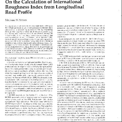
On The Calculation Of International Roughness Index -1501- Sayer 565cd
December 2019 69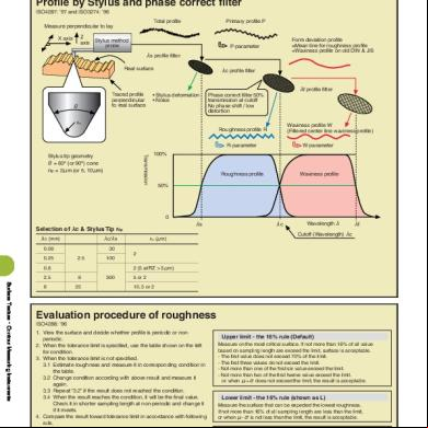
Explanation Of Surface Roughness 305n10
November 2019 106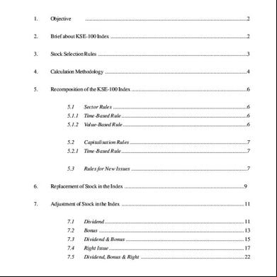
Calculation Methof Of Kse-100 Index 6o5131
November 2019 19
International Conference On The History Of Freemasonry s2b6p
October 2022 0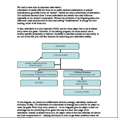
International Chess School-calculation 4n5k2o
November 2022 0
Color Rendering Index Calculation Pdf 2l2o4d
December 2019 72More Documents from "rendy" 3u4as

Ta 1 Bundel.pdf 2t4m1q
April 2020 48
Buku Manual Pondasi Tiang 225c5q
October 2020 0
Astm E1845 - Standard Practice For Calculating Pavement Macrotexture Mean Profile Depth.pdf 1q3u5v
January 2022 0
On The Calculation Of International Roughness Index -1501- Sayer 565cd
December 2019 69
Harga Laptop.xlsx 5yx5e
December 2019 85