Scour Depth 4p6k23
This document was ed by and they confirmed that they have the permission to share it. If you are author or own the copyright of this book, please report to us by using this report form. Report 3b7i
Overview 3e4r5l
& View Scour Depth as PDF for free.
More details w3441
- Words: 6,647
- Pages: 20
ESTIMATION OF SCOUR IN BRIDGE PIERS ON ALLUVIAL NON-COHESIVE SOIL BY DIFFERENT METHODS By S.K. Mazumder,∗ & Yashpal Kumar∗∗ SYNOPSIS IRC method of estimation of scour in bridge piers on alluvial non-cohesive soil is based on Lacey’s regime theory, which considers only two parameters, namely, discharge and mean size of bed materials. Actually scour is governed by many other parameters, which have been duly considered in the recently developed mathematical models. Total scour depth around piers is computed in five bridges by IRC method as well as four other popular mathematical models, namely Mellvile
& Coleman, Richardson & Davis (HEC - 18), Breussers &
Roudikivi (IAHR) and Kothyari – Garde – Ranga Raju. Total scour depth obtained by IRC method is found to be always more than that obtained by other mathematical models. The percentage excess total scour depth by IRC method with respect to that obtained by other mathematical models is found to vary from 2.5% to 275%. It is, however, not possible to conclude which of the models is the best in scour estimation unless prototype scour data under identical conditions are available from site for validation of the mathematical models most of which are developed on the basis of laboratory flume study. Limitation of Lacey’s method has been discussed and necessity of measuring scour at bridge sites has been emphasized. 1.
INTRODUCTION
Estimation of scour in bridge piers is extremely important as it helps in deciding their foundation level. Any under estimation of scour may result in failure of the bridge whereas over-estimation will lead to escalation of cost. Numerous bridges, all over the world, have
∗
Adviser, ICT Pvt. Ltd., A-8, Green Park, New Delhi - 16 Previously working as Generalt manager, ICT Pvt. Ltd.
∗∗
failed due to foundation failure of piers. One of the major causes of such foundation failure is due to scouring around pier during the age of high floods. The present practice being followed in India (IRC:78 ) is to estimate maximum scour level (MSL) at the bridge piers and fix the foundation level such that the anchoring below MSL is at least one third of the uned length of the pier. It may have to be lowered further due to inadequate bearing capacity of the sub-soil at the anchoring depth and also for ive pressure required for resisting the tractive force of vehicles moving above the bridge or from earthquake considerations etc. Total scour depth in a bridge pier consists of both general and localized scour. The general scour is due to the general morphologic behaviour of the river eg. degradation, meandering, braiding, confluence with another stream, cut-off formation etc. General scour will occur even though the bridge is not constructed. Localized scour has two components, namely, constriction scour due to restriction of waterway and local scour due to obstruction by pier and its foundation. A number of mathematical models have been developed for estimation of both general and localized scour. Melville (1984) Breussers (1977), Raudkivi (1983), Richardson and Davis (1995), Laursen (1956), Shen (1969) from abroad have done commendable study and developed scientific methods of scour estimation. In India, the mathematical models are developed by Garde (1996), Kothyari (1992a, b, 1993), Jain (1981), Gangadharaiah (1985) and others. Unfortunately, most of the mathematical models developed by using laboratory flume data are not proved or validated by field measurement of scour in prototype piers. IRC Codes {IRC-5(1998), IRC:SP-13(2004) and IRC:78(1980)} recommend use of Lacey’s (1930) equation for estimation of scour depth. However, Lacey’s method has several limitations. It is not scientific as it ignores many parameters which govern scour around bridge piers. Lacey did not consider sediment transport and threshold condition of bed motion. These limitations have been discussed in subsequent paragraphs. Objective of writing this paper is to estimate scour by different mathematical models as well as by Lacey’s method (as per IRC code) for some bridge piers located on alluvial noncohesive soil and then make a comparison between the scour depths obtained by the
(2)
mathematical models and those obtained by Lacey’s method. Due to non-availability of prototype scour data at bridge sites, it is however not possible to conclude which method is the most accurate. Necessity of scour observation at bridge sites has been discussed at the end of this paper.
2.
REVIEW
OF
DIFFERENT
METHODS
USED
FOR
SCOUR
COMPUTATIONS As already discussed, scour around piers can be sub-divided into three major components, namely, general scour, constriction scour and local scour. Methods of estimation of the different components of total scour in a bridge pier are briefly discussed in the following paragraphs.
2.1
General Scour
General scour is the scour which occurs irrespective of the presence of the bridge due to the morphological behaviour of a river, namely, the processes of aggradation and degradation of river bed, meandering, braiding, cut-off formation, confluence of streams upstream of bridge sites, etc. Long-term behaviour of a river in the vicinity of a bridge must be thoroughly explored to find the likely change in river bed elevation at the proposed bridge site. While degradation of river bed may result in foundation failure (if not properly ed for), general aggradation will cause rise in HFL, reducing free board and threatening the safety of the superstructure. The major causes of change in stream bed elevation can be attributed to human activities eg. construction of water retaining structures (like dams), diversion structures (like weirs and barrages), river improvement works (through dredging), river training works, encroachment of flood plain, change in catchment characteristics due to change in land use, mining of river bed, river bank erosion, land slide, etc. Lane (1957), Leopold and Wolman (1960), Lacey (1930), Blench (1969), Neill (1973), Diplas (1997), Yalin (1992), Garde and Rangaraju (2000), Chitale (1981) and many eminent river engineers have done commendable works to determine the general river behaviour to find dimensions of stable channel section (or regime section) of rivers for propagation of floods. Different concepts e.g. dominant discharge, minimum work, stream powers, etc. have been introduced. Apart from predicting the river bed forms (ripple, dune, antidane) and
(3)
plan forms (straight, meandering, braiding), most of them have tried to develop general relation of river width(B), depth of flow (D) and equilibrium slope (S) of streams for a given flow of water in a given bed material. In India, the most popular method of predicting the stable channel dimension is by using Lacey’s regime equations given below:B = P = 4.8 Q ½ ……………………….. 1/3
D = R = 0.473 (Q/f)
………………….
(1) (2)
S = 1/3340 (f5/3/ Q1/6 ) …………………… (3) f = 1.76 √d50…………………….
(4)
Knowing the design discharge, Q, and the type of bed materials (d50), one can predict the maximum mean depth of flow (D) that is likely to occur during the age of design flood (Q). D-value so obtained can be distributed all over the channel periphery, depending on whether the channel is straight, meandering or braided. Thus the general lowering/scouring of river bed with respect to low flow bed profile (usually surveyed during low flow period) can be obtained. In a meandering channel, however, the general degradation is highly non-uniform due to occurrence of secondary current in the river bend. There is concentration of flow towards the outer bank where deep scour occurs. On the inner bank side, there is deposition of scoured bed material causing rise in bed elevation. Fig. 1 shows plan and cross section of a typical meandering stream as it migrates. Rozovsky (1957), Thorne (1988), Oddgard (1989), Garde (2000), U.S.Army (1994)
Core
have
investigation
of made
to
Engineers in-depth find
the
characteristics of flow in bends and establish co-relation of bend scour with bank radius, degree of bend etc. In India, Lacey (1930) and Neill
(4)
(1973) have proposed coefficients (Ybs/R) for different types of Channels as given in Table-1 below. Ybs is the maximum scoured flow depth and R is hydraulic mean depth measured below HFL. Table 1 Effect of bend on maximum flow depth (Ybs) Coefficient Ybs/R
Channel Type
Lacey (1930) Greatly Constricted Section
1.00
--
Straight Channel
1.27
1.25
Moderate Bend
1.50
1.50
Severe Bend
1.75
1.75
Right Angled Bend
2.00
2.00
---
2.25
Alongside Cliffs & Walls
2.2
Neill (1973)
Constriction Scour
Constriction or contraction scour occurs in a bridge where the road or railway approach embankment restricts the normal waterway. It occurs also at such section where the bridge is sited at a natural contraction of a river usually selected as bridge site for reducing the cost of superstructure. Lowering of the bed occurs locally within the contracted reach (i.e. under the bridge) due to flow acceleration and increased velocity of flow. Excessive contraction of normal waterway (to reduce the cost of superstructure) increases construction cost of substructure due to excessive scour. It also causes several harmful effects, e.g. excessive afflux, longer backwater reach needing flood protection, sedimentation within the backwater reach due to reduction in sediment transporting capacity of the stream, meandering, flow instability, etc. (Mazumder 2002). There is also the possibility of outflanking of bridge approaches when the constriction is excessive (Mazumdar 2004). Estimation of constriction scour should be done depending on whether the bed is stable (rigid) or live (mobile). The bed becomes mobile (also known as live bed) when the mean velocity of flow(V) in the channel exceeds the critical velocity (Vc) or the bed shear stress (τo) exceeds the critical shear stress (τc) at which the streambed material just starts moving. Gill (1981), Laursen (1960) have contributed immensely for finding scour and flow characteristics due to restriction of waterway in a bridge.
(5)
For the case of clear water scour (τo < τc or V
6/7
……………… (5)
Where Y2 is the average depth including scour depth under the bridge in meter, Q2 is the total discharge through bridge in cumec, dm is effective mean diameter of the bed material in mm (dm = 1.25 d50), W2 is the average bottom width of river under the bridge in m and the constant (1.48) has a dimension (L-3/7). It is assumed that the scour continues to occur in the contracted reach until threshold condition is attained. Constriction scour depth (dsc) measured below original river bed is given by dsc = ( Y2- Yo), where dsc is the scour depth in m below bed and Yo is the original depth of flow in m at the contracted site before the construction of the bridge. Live bed scour (τo
>
τc or V>Vc) at a contracted section can be found by the equation
proposed by Richardson and Davis (1995- HEC-18) as follows: Y2/Y1 = (Q2/Q1m)6/7 (W1/W2)
K1
……………….(6)
where Y1 is the average depth of flow in the approach channel, Y2 is the average depth of flow in the main channel in the contracted section (including scour), Q1m is the discharge in the approach channel transporting sediments, Q2 is the total discharge ing under the bridge, K1 is a coefficient varying from 0.59 (for sediments transported mostly as bed load) to 0.69 (for sediment transport mostly in suspended form). W1 and W2 are the mean widths of the stream in the approach channel and the contracted section under the bridge respectively. The methods described above for finding constriction scour assume that the scour is uniform across the contracted section. Depending on the approach flow condition (with or without guide bank), the scour may not be uniform all over the section and may concentrate at some part of the cross-section. Different methods, as quantitative guidance, have been narrated by Melville (2000) for re-distribution of actual scour depth from a given mean depth of scour found from equation 5 & 6. 2.3
Local Scour
Local scour in bridge piers occur due to obstruction by pier and pier foundation and the consequent changes in the flow field around the piers. Because of variation in velocity from
(6)
top to bottom of a pier, the stagnation pressure head is the highest at top and lowest at the bottom of pier, thereby inducing a pressure gradient, since the potential head is highest at the top and lowest at the bottom of the pier. This causes a downward vertical flow impinging the bed. At the pier base, two horse-shoe vortices develop due to flow separation. It is primarily due to the vortex formation and the downward flow impinging on the bed that causes scour at the base of the pier as schematically shows in figure- 2. From non-dimensional analysis of the different parameters governing scour around a pier, it can be proved that
ds/b = f (V/Vc, y/b, b/d50,
σg,
Sh,
Al, G, Vt/b, V/ gb) ….(7) Fig. 2: Showing flow and scour patterns around a circular pier
First three represent flow intensity, flow shallowness and coarseness of sediments respectively, b is the thickness (size) of pier,
σg is the geometric non-uniformity coefficient
of sediments expressed as (d84/d16)0.5 , Sh. & Al are governed by the shape and alignment of piers, G represents the non-uniformity of approach flow and shape of cross-section of the approach channel, Vt/b is a non-dimensional time parameter representing the actual time of scour with respect to the time (te) required to attain equilibrium scour depth (ds), and the last parameter gives Froudes number of flow based on pier size. Thus the local scour around a pier is determined by a large number of parameters pertaining to flow, sediments, geometry of channel, pier geometry and alignment of piers with respect to flow, time available for scour with respect to equilibrium time etc. There are large number of research study on local scour around bridge piers all over the world and a large number of mathematical models have been evolved for estimating local scour around piers, principally on the basis of laboratory model study. Some of the most popular mathematical models which have been used to estimate scour depths in a few bridges (Table-2, given at the end) are briefly discussed in the following paragraphs.
(7)
3.
DIFFERENT
MATHEMATICAL
MODELS
USED
FOR
SCOUR
ESTIMATION Five of the most popular mathematical models including Lacey’s model are discussed briefly underneath:
3.1
Melville And Coleman Method
As already stated earlier, Melville and Coleman (2000) computed total scour depth by adding up the general scour, the constriction (or contraction) scour and local scour. Methods of estimating general and constriction scour which is almost the same in all the models have been already discussed. Local scour around piers(ds) below river bed has been expressed by Melville as ds = Kyb. K1 Kd . Ks . Kal . Kg . Kt……………………..(8) All other parameters except Kyb are non-dimensional and Kyb is having the same dimension as that of ds i.e. scour depth in meter. Kyb is depth-size or shallowness factor and is given by the relation Kyb = 2.4 b when b/y < 0.7, Kyb = 4.5y when b/y > 5 and Kyb = 2 √yb when 0.7 < y/b<5, K1 is flow intensity factor including sediment gradation, Kd is sediment size factor, Ks is pier shape factor, Kal is pier alignment factor, Kg is channel geometry factor, Kt is the time factor. For evaluation of the different K-values, the various mathematical equations and the design curves are given in the book “Bridge Scour” by Melville and Coleman (2000). The total scour depths computed by Melville and Coleman method for few bridges are given in Table 3(a) and 3(b).
3.2
HEC-18 Method (Richardson and Davis)
As in the case of Melville and Coleman method, HEC-18 (By Richardson and Davis, 1995) prescribes that the total scour should be separated as general scour, contraction scour and local scour. Computation of general and contraction scour depth are already discussed. For local scour estimation, Richardson and Davis (1995) recommend use of the following equation for both clear water and live bed scour depth, ds (measured below bed) , in of approach flow depth, y1 as
(8)
ds/y1 = 2K1. K2 . K3 . K4. (b/y1)0.65 . Fr1 0.43 ……………(9) Where K1 is correction factor for pier nose shape i.e. Ks in Mellville equation, K2 is correction factor for flow obliquity i.e. Kal in Melville equation, K3 is correction factor for bed condition i.e. plain bed, ripple and dune bed etc., K4 is the correction factor due to armoring of bed in non-uniform sediments, Fr1 is the approach flow Froude number directly upstream of pier given by the relation Fr1 = V1/
gy1 ………………………..(10)
Where V1 is the mean velocity of flow and y1 is the average flow depth directly upstream of piers. Values of K1, K2, K3, K4 are given in HEC-18 (Richardson and Davis – 1990) as well as in the book “Hydraulic Design Hand book” by Mays, (1999) in Chapter 15. Total scour depth for the few bridges computed by HEC-18 method are given in Table 3(a) and 3(b).
3.3
IAHR Method (Breussers & Raudkivi)
In this method too, the local scour at bridge pier is added up with general scour and constriction scour to obtain the maximum depth of total scour. Breussers and Raudkivi (1991) have differentiated between live bed scour and clear water scour up to threshold condition. Equilibrium condition reaches when the combined effect of the temporal mean shear stress, the weight component and the turbulent forces are in equilibrium everywhere within the scour hole. For live bed scour, an excess shear stress (τo - τc ) must exist for transport of the sediments through the scour hole. However, the particles on the surface of the equilibrium scour hole may occasionally move but are not carried away. For clear water local scour (dse) when u < uc , or V < Vc * * dse/b = 2.3 Kσ K(b/d50) Kd Ks Kα ……………….(11) and for live bed scour when u > uc , or V>Vc, the equation is * * dse/b = X. K(b/d50). Kd. Ks Kα ……………….(12) Here dsc is the equilibrium scour depth measured below river bed, Kσ is a coefficient for gradation of sediment, K(b/d50) is a coefficient owing to size of sediments with respect to pier size ‘b’, Kd is a factor due to depth of flow or flow shallowness, Ks is shape factor, Kα is the pier alignment factor. Maximum value of X is 2.3 when V > 4Vc. When Vc
<4Vc, value of
(9)
X varies from 2 to 2.30 for uniform sediments (σg ≤1.3) and “X”varies from 0.5 to 2.0 for non-uniform sediments (σg >1.3). Values of the different coefficients are available from graphs given in the book “Scouring” by Breussers and Raudikivi (1991). Total scour depth computed by IAHR method for few bridges are given in Table 3(a) and 3(b).
3.4
Kothyari – Garde - Rangaraju Method
Based on the analysis of extensive laboratory data collected for uniform, non-uniform and stratified sediments, steady and unsteady flows, the following mathematical equations have been proposed by Kothyari, Garde and Ranga Raju (1992) for estimation of local scour under clear water and live bed conditions when the flow is parallel to pier axis without any obliquity. For clear water scour depth (dse) measured below bed : dse/d50 = 0.66(b/d50)0.75
{(D/d50)0.16} {(V2-V2c)ρ/∆ γs.d50}.α -0.30……..(13)
For live or mobile bed scour : dse/d50 = 0.88 (b/d50) 0.67 (D/d50)0.4 α.-0.3 ………………………..(14) Where D is the average flow depth, d50 is the mean sediment size, V is the mean flow velocity, ∆ γs =( γs –γf ), γs and γf are the unit weights of sediments and water respectively. ρ is the density of water, α = (B-b)/ B, B is the centre to centre spacing of piers, b is the pier thickness, V is the actual mean velocity of flow under the bridge, Vc is the mean critical velocity of flow for the given bed material at threshold condition expressed as Vc2 ρ/ γs.d50 = 1.2 (b/d50)-0.11 (D/d50)0.16 ……………..(15) Total scour depth as found by adding up general scour and constriction scour with local scour found from equations 13 and 14 for few bridges are given in Table 3(a) and 3(b) 3.5
IRC Method (Lacey/Inglis)
IRC:5, IRC:SP:13 & IRC 78, published by Indian Roads Congress (IRC), recommend use of Lacey’s (1930) equations for estimating scour depth in a pier. Unlike the other mathematical models, IRC method does not distinguish between local scour, constriction scour and general scour. The total scour depth (measured below HFL) is assumed to be 2 times Lacey’s R,
(10)
given by the equations 16 and 17 below, as per the prototype scour observations made by Inglis (1949) at bridge sites. R = 0.473(Q/f)1/3, when L/W > 1 …………………………………..(16) R = 1.34(q2/f)1/3, when L/W <1,
…………………….……………(17)
Here, Q is the design discharge in cumec, R is the regime depth, q is the discharge intensity i.e. m3/s/m i.e. Q/L and f is Lacey’s silt factor given by equation (4), L is the clear waterway under the bridge and W is the mean width of waterway in the approach channel (regime width) corresponding to design discharge Q. IRC 78 recommends that bridge pier foundation should be designed for an additional flow varying from 10% (for large catchment) to 30% (for small catchments) over and above the design flood discharge of 50 years return period. With the above assumptions, the maximum scour depth for piers (recommended as 2R below design high flood level corresponding to the design discharge) are computed for the different bridges and are given in Table 3(a) and 3(b).
4.
LIMITATIONS OF LACEY’S METHOD
Lacey’s equations are applicable for finding approximate dimensions of a stable channel which is said to be in regime state. Inglis (1949) measured actual scour depths in bridge piers, abutments, guide bundhs etc. and recommended that the actual scour depth may be obtained by multiplying Lacey’s regime depth {R=0.473(Q/f)1/3}by the following factors. At nose of pier At u/s head of guide baundh –
– 2R. 2.75R .
At the shank of guide baundh – 1.5R. Since these factors were determined with respect to field observations in a limited number of structures, they should not be generalized. Lacey’s method of finding scour depth (R) and the maximum scour depth in bridge piers is not scientific due to the following reasons:(i)
Lacey’s formulae were developed for stable irrigation channels with fine incoherent alluvial soils which can be as easily scoured as deposited. Such ideal conditions do not exist at all the bridge sites. With the development of bed load transport theory,
(11)
Ning Chien (1957) proved that Lacey’s silt factor (f) can be expressed in different forms as: f(V,R) = 2.52 V2/R
……………………….(18)
f(R,S) = 291 R1/3 .S2/3
………………………(19)
f(R,S,V) = 3127 RS/V
….……………………(20)
comparing Lacey’s equation with Einstein’s (1953) bed load equation, it can be shown that in FPS unit Lacey’s silt factor (f) is given by the relation: 1.37f = {(qs/q).C4 d501.5 (Ss – 1)5/2 g1/2/ 40(Gq)}………………(21) where qs and q are the sediment and water transport rates per unit width, C is Chezy’s constant, G is Stoke’s constant in the fall velocity (w) relation: w=G{gd50(Ss-1)}1/2 (ii)
…………….(22)
In Lacey’s method of computations, only two parameters e.g. flow (Q or q) and mean sediment size (d50) are considered whereas actual scour around piers is governed by several parameters e.g. flow parameters (velocity, depth, turbulence, flow obliquity etc.), geometric parameters of pier and its foundation (e.g. size, shape, length of pier location of pier …..etc.), sediment parameters (e.g. size, coarseness and nonuniformity, layering, armoring of bed etc.) channel geometry (e.g. nature of crosssection, flood plain encroachment, extent of constriction, asymmetry of bridge opening with respect to approach flow, type of bed form and plan form of the stream etc.) hydrological parameters (e.g. flood peak and its duration, nature of flood hydrograph etc.)
(iii)
In Lacey/Inglis equation, no consideration has been made regarding sediment transport and bed movement at high flows. As such Lacey / Inglish equation results in increased scour depth with increasing mean velocity of flow or in other word increasing discharge. However, it is well established now, all over the world, that the maximum scour is attained when the mean velocity of flow is equal to the critical velocity at which the bed movement commences for a given bed material. i.e. at threshold condition. Once the bed movement starts after the mean velocity exceeds the critical velocity, the scour depth reduces since the scour hole starts receiving sediments from upstream. In fact, the maximum equilibrium scour depth in a pier under mobile bed condition is found to be slightly less than the maximum scour depth observed at threshold or critical stage. (Fig. 3)
(12)
Once
the equilibrium
scour depth is attained, the scour
depth
remains
constant even though there may be further increase in mean
velocity
or
discharge. This fact is not reflected in Lacey/Inglis equation
wherein
scour
goes on increasing with increase in discharge.
5.
Fig. 3: Showing local scour depth variation with sediment nonuniformity and illustrating clear-water and livebed scour in bridge piers.
COMPARISON OF SCOUR DEPTHS COMPUTED BY DIFFERENT
METHODS Scour depths are computed by different methods as discussed above for five numbers of bridges, salient features of which are given in Table-2. Maximum total scour depth (below HFL) i.e. the sum total of general scoured flow depth (below HFL), constriction scour depth and local scour depth are given in Table 3(a) and Table 3(b). Since Lacey’s method, (as adopted in IRC: SP-13, IRC-5 and IRC-78) do not distinguish between local and general scour, only total scour depth below HFL is given in Table 3(a) and 3(b). Because of space limitation, details of computations are not given in the paper. In Table 3(a), the general scoured flow depth is taken as the average of regime depths found by Lacey’s and Blench’s formula. In Table 3(b), however, the general scoured flow depth is taken as the mean flow depth measured above the mean bed level (i.e. HFL-Mean Bed Level) as obtained from the bed profile during low flow period, assuming that the bed profile of the stream remains the same during low and high flow periods. From the above tables, it is seen that IRC method (from Lacey’s theory) overestimates scour compared to that found by other mathematical models. Percentage excess scour as obtained from Lacey (or IRC) method in comparison to that obtained by the different mathematical models is also indicated in both the tables (figures given in brackets). The percentage excess scour is found to vary from 2.4% to 90% in able 3(a). In table 3(b), where the general scoured
(13)
flow depth is assumed to be the same as the mean flow depth (measured from HFL to the mean bed level as obtained during low flow period), the percentage excess scour by IRC method is found to vary from 10.2% to as high as 275.2%. Such wide variation occurs as Lacey’s method is an empirical method and it does not consider the various parameters governing scour.
6.
NECESSITY OF SCOUR MEASUREMENT AT BRIDGE SITES
Although it is apparent from table 3(a) and 3(b) that there is a large percentage variation in scour depth obtained by IRC method with respect to those found by different mathematical models, it cannot be ascertained which method is the best for scour computation. Most of the mathematical models are developed by using data obtained from laboratory flume study and there may be considerable error between model and prototype scour due to scale effect as well as disparity in flow fields in models and prototypes. It is extremely difficult to reproduce the prototype flow and bed condition in the physical model. It is essential, therefore, that before the use of any mathematical model for computing scour in bridge piers, the model must be proved or validated by means of actual prototype scour observations under identical condition of flow and other parameters used in scour estimation. It is highly unfortunate that even though a large amount of public money is being spent in bridge construction, hardly there is any effort to collect, preserve and systematically analyze precious scour data from bridge sites for the validation of mathematical models which have been developed in a scientific manner and are in use in most of the developed countries in the world. Afterall, Lacey’s method being currently used for scour estimation by IRC, RDSO, BIS codes, etc. is an empirical method and it is advisable to replace empiricism by a more scientific and rational approach developed by gifted research workers in India and abroad.
7.
SUMMARY AND CONCLUSIONS
Estimation of scour around bridge piers is a routine work for foundation design. The current method of scour estimation as prescribed in IRC, RDSO and IS Codes (used in India) is based on Lacey’s regime theory developed in 1930 . Lacey’s method has several limitations as it ignores many important parameters like size of pier and its foundation etc. Several mathematical models have been developed over the years for precise estimation of general
(14)
scour, constriction scour and local scour. Scour around piers in 5 bridges are computed using the five different mathematical models of Melville & Coleman, Richardson & Davis (HEC-18), Breussers & Raudkivi (IAHR), Kothyari-Garde and Rangaraju and Lacey/Inglis. Total depths of scour found from first four models have been compared with scour depths found by Lacey’s method adopted in India. There is a lot of variation in total scour depths. Percentage excess scour found by
Lacey’s method with respect to other mathematical
models range between 2.4% to 90% in table 2a where general scour depth is taken as regime depth of flow. The corresponding figures are found to be 10.2% to 275.2% in table 2b where the general scour is taken as the mean flow depth measured from HFL to mean bed level (observed during low flow). The total scour depths estimated by the different mathematical models (other than Lacey) are nearly the same. It is, however, difficult to conclude which mathematical model gives the best result unless the results are compared with actual scour measurement in prototype at different bridge sites. Measurement of scour at site during the age of high floods is extremely important for validation of mathematical models most of which have been developed on the basis of scour data obtained in laboratory flumes.
8.
ACKNOWLEDGEMENT
Authors expresses their deep sense of gratitude to ICT authorities for providing all the help, and encouragement. All the help received from Ms. Rajni Dhiman, Deputy Manager of hydrology division, Shri S.P.Rastogi, Head and Shri D.K.Rastogi, GM of bridge division are gratefully acknowledged. Last but not the least, they thank Mr. Neeraj for neatly typing and organizing the paper. REFERENCES Blench, T. (1969) “Mobile Bed Fluviology”, University of Alberta Press, Edmonton, Canada. Breussers, H.N.C., Nicollet, G. and Shen, H.W. (1977), “Local Scour around cylindrical Piers’, Journal of Hydraulic Research (JHR), I.A.H.R., 15(3), P. 211-25, Breussers, HNC and Randviki, A.J. (1991) “Scouring” , Chapter-5 “Scour at Bridge Piers” A.A. Balkema Pub., IAHR Hydraulic Structures Design Manual. Chitale, S.V.(1981), “Shape and Mobility of River Meanders”, Proc. XIX Congress of IAHR, Volume 2, New Delhi P. 281-286. Diplas P. and Vigilar, G.G. (1992), “Hydraulic Geometry of Threshold Channels” JHE, A.S.C.E., 118(40, P. 597-614 Einstein, H.A. (1953), “Formulae for the transportation of Bed Load”, Trans. A.S.C.E.,
(15)
Vol. 107 Gangadarhiah, T., Muzzammil, M. and Subramanya, K (1985) “Vortex Strength Approach to Scour Depth Prediction Around Bridge Piers”, Proc. 2nd Int. Workshop on Alluvial River Problems held at University of Roorkee, Roorkee, India. Garde, R.J. and Kothyari, U.C. (1996) “State of Art Report on Scour around Bridge Piers”, Indian Institute of Bridge Engineers, Mumbai, India. Garde, R.J. and Ranga Raju, K.G.(2000) “Mechanics of Sediment Transport and Alluvial Stream Problems”, 3rd Ed., New Age Int. Pub. Pvt. Ltd. New Delhi. Gill, M.A.(1981) “Bed Erosion in Rectangular Long Contraction” JHE, A.S.C.E. 107(HY3), P. 273-294. IRC:5 (1998) “Standard Specifications and Code of Practice for Road Bridges – Section 1” Published by Indian Roads Congress, R.K.Puram, New Delhi. IRC:78: (1980) “Standard Specifications and Code of Practice for Bridges – Section VII Foundation and Substructures, Part-I, General Features of Design”. Published by Indian Road Congress, New Delhi. IRC:SP:13(2004) “Guidelines for the Design of Small Bridges and Culverts”, Published by Indian Roads Congress, New Delhi. Jain, S.C. (1981) “Maximum Clear Water Scour around Cylindrical Piers”, JHE, A.S.C.E., 107(5), P. 611-625. Johanson, P.A. (1995), “Comparison of Pier Scour Equation using Field Data”, JHE, A.S.C.E. 121(8), P. 626-630. Kothyari, U.C. (1993) “Scour Around Bridge Piers” – Theme Paper, Proc. Workshop on “River Scour” org. by CBI&P at Varanasi, India, April 28-29. Kothyari, U.C. Garde, R.J. and Ranga Raju, K.G. (1992-b), “Live Bed Scour around Cylindrical Bridge Piers”, JHR, IAHR, 30(5), PP 701-715. Kothyari, U.C., Garde, R.J. and Ranga Raju, K.G. (1992a) “Temporal Variation of Scour Around Circular Bridge Piers”, JHE, A.S.C.E., 118(8), PP 1091-1106. Lacey, G.(1930) “Stable Channels in Alluvium” Paper 4736, Proc. Of Institution of Civil Engineers, Vol. 229, William Clowes & Sons Ltd., London, U.K. P. 259-292. Lane (1957), “A study of the shape of channels formed by Natural Streams flowing in Erodible Material”, M.R.D. Sediment Series No. 9, U.S. Army Corps. Of Engineers, Missouri River. Laursen, E.M. (1981) “Scour at Bridge Crossings”, JHE, A.S.C.E. 86(2), P. 39-54. Laursen, E.M. and Toch, A. (1956), “Scour Around Bridge Piers and Abutments”, Ames, Iowa, U.S.A. Leopold, L.B. and Wolman, M.G. (1960) “River Meanders”, Geological Soc. Of America, Bulletin, Vol. 71. Mazumdar S.K. (2004), “River Behaviour Upstream and Downstream of Hydraulic Structures” Proc. Int. Conf. on Hydraulic Engineering : Research and Practice, organized by Deptt. Of
(16)
Civil Engineering, IIT, Roorkee, Vol. I, P.253-263. Mazumdar S.K., Rastogi S.P. and Hmar, Rofel (2002) “Restriction of Waterway under Bridges” J. of Indian Highways, Vol. 30, No. 11, Nov., Indian Roads Congress, New Delhi. Mazumder, S.K. and Dhiman, Rajni “Computation of Afflux in Bridges with particular reference a National Highway” Proc. HYDRO-2003, Pune (CWPRS), Dec 26-27.
Mays,Larry, W..(1999) “Hydraulic Design Handbook”McGraw – Hill Publication Melville, B.W. (1984), “Live Bed Scour at Bridge Sites”, Journal of hydraulic Engineering (JHE), A.S.C.E., 110(9), P.234-1247 Melville, B.W. (1997) “Bridge and Abutment” scour – An Integrated Approach”, JHE, A.S.C.E., 123(2), P 125-136. Melville, B.W. and Coleman, S.E.(2000) “Bridge Scour”, Water Resources Publications, LLC Neill, C.R. (1973), “Guide to Bridge Hydraulics” Roads and Transportation Association of Canada, University of Toronto Press, Toronto, Canada. Ning Chien (1957), “A concept of Regime Theory”, Trans. A.S.C.E., Vo. 122. Oddgard, A.J. and Wang, Y. (1989a) “River Meander Model I : Development, (1989) River Meander Model II: Applications JHE, A.S.C.E., 115(11), P. 1435-1464. Raudkivi, A.J. and Ettema, R. (1983), “Clear Water Scour at Cylindrical Piers”, JHE, A.S.C.E., 109(3) P.339-350. Richardson, E.V. and Davis, S.R. (1995), “Evaluating Scour at Bridges”, Report No. FHWAIP-90-017, Hydraulic Engineering Circular No. 18 (HEC-18), Third Edition, Office of Technology Applications, HTA-22, Federal Highway istration, U.S. Department of Transportation, Washington D.C., U.S.A., Richardson and Mays (1999) “Hydraulic Design Handbook” Mc Graw-Hill Company, Chapter 15. Rozovski, J.L. (1957), “Flow of Water in Bends of Open Channels”, Academy of Sciences of the Ukranian SSR, Translated in English by Prushansky, Y., Israel Programme of Scientific Translation. Shen, H.W., Schneider, V.R. and Karaki, S.S. (1969) “Local Scour Around Bridge Piers”, JHE, A.S.C.E., 95 (HYL) P. 1919-1940. Thorne, C.R. and Osman, A.M. (1988) “River Bank Stability Analysis:II:Applications”: JHE, A.S.C.E., 114(2), P. 151-172. U.S.Army Corps of Engineers (1994), “Hydraulic Design of Flood Control Channels” EM 1110-2-1601’, U.S.Army Corps of Engineers, Washington, D.C., USA Yalin, M.S. (1992), “River Mechanics”, Pergaunon Press, New York, U.S.A.
(17)
Annexure-II Table -2 : Different Parameters for Computing Scour in Bridge Piers Name of z Stream (NH-No)
Hydrologic Parameters (for Design of Bridges)
Stream and Sediment Parameters Averag NonMean Hydrauli e bed Lowest Uniform width of c mean slope S. d50 Bed ity approac depth Value of (mm) Level Coeff. h Water (m) (m) H in way (m) (σp) S =1: H
Chambal 1 (NH-3) Saryu 2 (NH-28) Raidak-I 3(NH31C) Raidak-II (NH31C) Sankosh 5(NH31C)
Foundation Parameters
Pier Parameters
Clear Design Water discharge of 50 yrs Design way return HFL (m) under Bridge period (m) (cumec)
Shape
Size, Flow Type b (m) obliguity
Size
1200
23.08
12,222
0.17
1.97
109.00
45000.00 145.53
810
Circular
3.5
0
o
Well
9.0
1440
3.44
3,662
0.30
5.48
82.45
28316.00
93.50
1228
Wall Type
1.2
0o
Well
7.0
365
4.98
2,160
1.80
3.42
43.53
3376.00
50.73
204
Circular
2.5
0
o
Well
6.0
365
4.78
979
3.65
3.54
41.40
3390.00
50.57
205
Circular
2.9
0o
Well
6.0
350
4.69
633
2.40
3.74
43.67
5498.00
49.10
336
Circular
2.9
0
o
Well
6.0
(18)
Table - 3(a) - SCOUR DEPTHS COMPUTED BY DIFFERENT METHODS (Assuming that the low water bed profile develops to regime profile during age of design flood)
Sl.No.
Name of River Crossing (NH No.)
Maximum scour depth (m) in Bridge Piers computed by different methods Local scour below bed and total scour below HFL (i.e., sum total of general scour, consriction scour and local scour) General ConstrictTotal scour scoured depth ion scour depth by below HFL (As Melville & Richardson & Breussers & Kothyari, Garde depth below Lacey (IRC per Regime Coleman Davis (HEC-18) Raudkivi (IAHR) & Ranga Raju mean bed level method) theory)
1
Chambal (NH-3)
23.80
6.83
46.27
Local 7.20
Total Local 37.83 6.23 (22.3%)
Total Local 36.86 6.90 (25.6%)
Total Local 37.53 13.18 (23.4%)
Total 43.81 (5.6%)
2
Saryu (NH-28)
10.20
1.10
26.04
2.88
14.18 (83.6%)
2.86
14.16 (84.0%)
2.40
13.7 (90.0%)
4.51
15.81 (64.6%)
3
Raidak - 1 (NH31C)
6.23
2.84
15.57
6.00
15.07 (3.2%)
4.26
13.33 (17.0%)
3.12
12.19 (28.8%)
6.12
15.19 (2.4%)
4
Raidak-II (NH-31C)
5.97
3.41
16.43
6.66
16.04 (2.4%)
4.75
14.13 (16.3%)
2.70
12.08 (36.0%)
6.29
15.67 (4.9%)
5
Sankosh (NH1.C)
5.86
0.15
13.70
6.96
12.97 (5.6%)
5.46
11.47 (19.4%)
3.50
9.51 (44.0%)
5.73
11.74 (16.7%)
Note:(i) All scour depths are in meter. Total scour depth is from Design HFL to maximum scour level (MSL) around the pier. Constriction and local scour depths are below mean bed level of the stream. (ii) Figures in brackets indicate percentage excess total scour by Lacey's (IRC) method with respect to other methods (iii) General scoured depth of flow is computed as the average of regime flow depths computed by Lacey's and Blench's theories
(19)
Table - 3(b) - SCOUR DEPTHS COMPUTED BY DIFFERENT METHODS (Assuming that the low water bed profile remains unchaged during the age of design flood)
Sl. No.
Name of River Crossing (NH No.)
Maximum scour depths (m) in Bridge piers computed by different methods Local scour below bed and total scour below HFL (I.e. sum of mean depth, constriction & local scour) by different methods Constriction Total scour depth Mean Depth of by Lacey (IRC scour depth below Melville & Richardson & Breussers & Kothyari Garde flow below HFL method) mean bed level Coleman Davis (HEC-18) Raudkivi (IAHR) & Ranga Raju Local Total Local Total Local Total Local Total 17.92 6.83 46.27 7.20 31.95 6.23 30.98 6.90 31.65 13.18 37.93 (44.8%) (49.5%) (46.2%) (22.0%)
1
Chambal (NH-3)
2
Saryu (NH-28)
3.44
1.10
26.04
2.88
7.42 (250.9%)
2.86
7.40 (251.9%)
2.40
6.94 (275.2%)
4.51
9.05 (187.7%)
3
Raidak - 1 (NH-31C)
4.88
2.84
15.57
6.00
13.72 (13.4%)
4.26
11.98 (30.0%)
3.12
10.84 (43.6%)
6.12
13.84 (12.5%)
4
Raidak-II (NH-31C)
4.76
3.41
16.43
6.66
14.83 (10.8%)
4.76
12.93 (27.1%)
2.70
10.87 (51.1%)
6.29
14.46 (13.6%)
5
Sankosh (NH1.C)
4.69
0.15
13.71
6.96
11.80 (16.2%)
5.46
10.3 (33.1%)
3.50
8.34 (64.4%)
5.73
10.57 (29.3%)
Note:(i) All scour depths are in meter. Total scour depth is from Design HFL to maximum scour level (MSL) around the pier. Constriction and local scour depths are below mean bed level of the stream (ii) Figures in brackets indicate percentage excess total scour by Lacey's (IRC) method with respect to other methods (iii) Mean depth of flow is from design HFL to mean bed level of the stream assuming that the bed profile observed during low flow remains unchanged during the age of design flood
(20)
& Coleman, Richardson & Davis (HEC - 18), Breussers &
Roudikivi (IAHR) and Kothyari – Garde – Ranga Raju. Total scour depth obtained by IRC method is found to be always more than that obtained by other mathematical models. The percentage excess total scour depth by IRC method with respect to that obtained by other mathematical models is found to vary from 2.5% to 275%. It is, however, not possible to conclude which of the models is the best in scour estimation unless prototype scour data under identical conditions are available from site for validation of the mathematical models most of which are developed on the basis of laboratory flume study. Limitation of Lacey’s method has been discussed and necessity of measuring scour at bridge sites has been emphasized. 1.
INTRODUCTION
Estimation of scour in bridge piers is extremely important as it helps in deciding their foundation level. Any under estimation of scour may result in failure of the bridge whereas over-estimation will lead to escalation of cost. Numerous bridges, all over the world, have
∗
Adviser, ICT Pvt. Ltd., A-8, Green Park, New Delhi - 16 Previously working as Generalt manager, ICT Pvt. Ltd.
∗∗
failed due to foundation failure of piers. One of the major causes of such foundation failure is due to scouring around pier during the age of high floods. The present practice being followed in India (IRC:78 ) is to estimate maximum scour level (MSL) at the bridge piers and fix the foundation level such that the anchoring below MSL is at least one third of the uned length of the pier. It may have to be lowered further due to inadequate bearing capacity of the sub-soil at the anchoring depth and also for ive pressure required for resisting the tractive force of vehicles moving above the bridge or from earthquake considerations etc. Total scour depth in a bridge pier consists of both general and localized scour. The general scour is due to the general morphologic behaviour of the river eg. degradation, meandering, braiding, confluence with another stream, cut-off formation etc. General scour will occur even though the bridge is not constructed. Localized scour has two components, namely, constriction scour due to restriction of waterway and local scour due to obstruction by pier and its foundation. A number of mathematical models have been developed for estimation of both general and localized scour. Melville (1984) Breussers (1977), Raudkivi (1983), Richardson and Davis (1995), Laursen (1956), Shen (1969) from abroad have done commendable study and developed scientific methods of scour estimation. In India, the mathematical models are developed by Garde (1996), Kothyari (1992a, b, 1993), Jain (1981), Gangadharaiah (1985) and others. Unfortunately, most of the mathematical models developed by using laboratory flume data are not proved or validated by field measurement of scour in prototype piers. IRC Codes {IRC-5(1998), IRC:SP-13(2004) and IRC:78(1980)} recommend use of Lacey’s (1930) equation for estimation of scour depth. However, Lacey’s method has several limitations. It is not scientific as it ignores many parameters which govern scour around bridge piers. Lacey did not consider sediment transport and threshold condition of bed motion. These limitations have been discussed in subsequent paragraphs. Objective of writing this paper is to estimate scour by different mathematical models as well as by Lacey’s method (as per IRC code) for some bridge piers located on alluvial noncohesive soil and then make a comparison between the scour depths obtained by the
(2)
mathematical models and those obtained by Lacey’s method. Due to non-availability of prototype scour data at bridge sites, it is however not possible to conclude which method is the most accurate. Necessity of scour observation at bridge sites has been discussed at the end of this paper.
2.
REVIEW
OF
DIFFERENT
METHODS
USED
FOR
SCOUR
COMPUTATIONS As already discussed, scour around piers can be sub-divided into three major components, namely, general scour, constriction scour and local scour. Methods of estimation of the different components of total scour in a bridge pier are briefly discussed in the following paragraphs.
2.1
General Scour
General scour is the scour which occurs irrespective of the presence of the bridge due to the morphological behaviour of a river, namely, the processes of aggradation and degradation of river bed, meandering, braiding, cut-off formation, confluence of streams upstream of bridge sites, etc. Long-term behaviour of a river in the vicinity of a bridge must be thoroughly explored to find the likely change in river bed elevation at the proposed bridge site. While degradation of river bed may result in foundation failure (if not properly ed for), general aggradation will cause rise in HFL, reducing free board and threatening the safety of the superstructure. The major causes of change in stream bed elevation can be attributed to human activities eg. construction of water retaining structures (like dams), diversion structures (like weirs and barrages), river improvement works (through dredging), river training works, encroachment of flood plain, change in catchment characteristics due to change in land use, mining of river bed, river bank erosion, land slide, etc. Lane (1957), Leopold and Wolman (1960), Lacey (1930), Blench (1969), Neill (1973), Diplas (1997), Yalin (1992), Garde and Rangaraju (2000), Chitale (1981) and many eminent river engineers have done commendable works to determine the general river behaviour to find dimensions of stable channel section (or regime section) of rivers for propagation of floods. Different concepts e.g. dominant discharge, minimum work, stream powers, etc. have been introduced. Apart from predicting the river bed forms (ripple, dune, antidane) and
(3)
plan forms (straight, meandering, braiding), most of them have tried to develop general relation of river width(B), depth of flow (D) and equilibrium slope (S) of streams for a given flow of water in a given bed material. In India, the most popular method of predicting the stable channel dimension is by using Lacey’s regime equations given below:B = P = 4.8 Q ½ ……………………….. 1/3
D = R = 0.473 (Q/f)
………………….
(1) (2)
S = 1/3340 (f5/3/ Q1/6 ) …………………… (3) f = 1.76 √d50…………………….
(4)
Knowing the design discharge, Q, and the type of bed materials (d50), one can predict the maximum mean depth of flow (D) that is likely to occur during the age of design flood (Q). D-value so obtained can be distributed all over the channel periphery, depending on whether the channel is straight, meandering or braided. Thus the general lowering/scouring of river bed with respect to low flow bed profile (usually surveyed during low flow period) can be obtained. In a meandering channel, however, the general degradation is highly non-uniform due to occurrence of secondary current in the river bend. There is concentration of flow towards the outer bank where deep scour occurs. On the inner bank side, there is deposition of scoured bed material causing rise in bed elevation. Fig. 1 shows plan and cross section of a typical meandering stream as it migrates. Rozovsky (1957), Thorne (1988), Oddgard (1989), Garde (2000), U.S.Army (1994)
Core
have
investigation
of made
to
Engineers in-depth find
the
characteristics of flow in bends and establish co-relation of bend scour with bank radius, degree of bend etc. In India, Lacey (1930) and Neill
(4)
(1973) have proposed coefficients (Ybs/R) for different types of Channels as given in Table-1 below. Ybs is the maximum scoured flow depth and R is hydraulic mean depth measured below HFL. Table 1 Effect of bend on maximum flow depth (Ybs) Coefficient Ybs/R
Channel Type
Lacey (1930) Greatly Constricted Section
1.00
--
Straight Channel
1.27
1.25
Moderate Bend
1.50
1.50
Severe Bend
1.75
1.75
Right Angled Bend
2.00
2.00
---
2.25
Alongside Cliffs & Walls
2.2
Neill (1973)
Constriction Scour
Constriction or contraction scour occurs in a bridge where the road or railway approach embankment restricts the normal waterway. It occurs also at such section where the bridge is sited at a natural contraction of a river usually selected as bridge site for reducing the cost of superstructure. Lowering of the bed occurs locally within the contracted reach (i.e. under the bridge) due to flow acceleration and increased velocity of flow. Excessive contraction of normal waterway (to reduce the cost of superstructure) increases construction cost of substructure due to excessive scour. It also causes several harmful effects, e.g. excessive afflux, longer backwater reach needing flood protection, sedimentation within the backwater reach due to reduction in sediment transporting capacity of the stream, meandering, flow instability, etc. (Mazumder 2002). There is also the possibility of outflanking of bridge approaches when the constriction is excessive (Mazumdar 2004). Estimation of constriction scour should be done depending on whether the bed is stable (rigid) or live (mobile). The bed becomes mobile (also known as live bed) when the mean velocity of flow(V) in the channel exceeds the critical velocity (Vc) or the bed shear stress (τo) exceeds the critical shear stress (τc) at which the streambed material just starts moving. Gill (1981), Laursen (1960) have contributed immensely for finding scour and flow characteristics due to restriction of waterway in a bridge.
(5)
For the case of clear water scour (τo < τc or V
6/7
……………… (5)
Where Y2 is the average depth including scour depth under the bridge in meter, Q2 is the total discharge through bridge in cumec, dm is effective mean diameter of the bed material in mm (dm = 1.25 d50), W2 is the average bottom width of river under the bridge in m and the constant (1.48) has a dimension (L-3/7). It is assumed that the scour continues to occur in the contracted reach until threshold condition is attained. Constriction scour depth (dsc) measured below original river bed is given by dsc = ( Y2- Yo), where dsc is the scour depth in m below bed and Yo is the original depth of flow in m at the contracted site before the construction of the bridge. Live bed scour (τo
>
τc or V>Vc) at a contracted section can be found by the equation
proposed by Richardson and Davis (1995- HEC-18) as follows: Y2/Y1 = (Q2/Q1m)6/7 (W1/W2)
K1
……………….(6)
where Y1 is the average depth of flow in the approach channel, Y2 is the average depth of flow in the main channel in the contracted section (including scour), Q1m is the discharge in the approach channel transporting sediments, Q2 is the total discharge ing under the bridge, K1 is a coefficient varying from 0.59 (for sediments transported mostly as bed load) to 0.69 (for sediment transport mostly in suspended form). W1 and W2 are the mean widths of the stream in the approach channel and the contracted section under the bridge respectively. The methods described above for finding constriction scour assume that the scour is uniform across the contracted section. Depending on the approach flow condition (with or without guide bank), the scour may not be uniform all over the section and may concentrate at some part of the cross-section. Different methods, as quantitative guidance, have been narrated by Melville (2000) for re-distribution of actual scour depth from a given mean depth of scour found from equation 5 & 6. 2.3
Local Scour
Local scour in bridge piers occur due to obstruction by pier and pier foundation and the consequent changes in the flow field around the piers. Because of variation in velocity from
(6)
top to bottom of a pier, the stagnation pressure head is the highest at top and lowest at the bottom of pier, thereby inducing a pressure gradient, since the potential head is highest at the top and lowest at the bottom of the pier. This causes a downward vertical flow impinging the bed. At the pier base, two horse-shoe vortices develop due to flow separation. It is primarily due to the vortex formation and the downward flow impinging on the bed that causes scour at the base of the pier as schematically shows in figure- 2. From non-dimensional analysis of the different parameters governing scour around a pier, it can be proved that
ds/b = f (V/Vc, y/b, b/d50,
σg,
Sh,
Al, G, Vt/b, V/ gb) ….(7) Fig. 2: Showing flow and scour patterns around a circular pier
First three represent flow intensity, flow shallowness and coarseness of sediments respectively, b is the thickness (size) of pier,
σg is the geometric non-uniformity coefficient
of sediments expressed as (d84/d16)0.5 , Sh. & Al are governed by the shape and alignment of piers, G represents the non-uniformity of approach flow and shape of cross-section of the approach channel, Vt/b is a non-dimensional time parameter representing the actual time of scour with respect to the time (te) required to attain equilibrium scour depth (ds), and the last parameter gives Froudes number of flow based on pier size. Thus the local scour around a pier is determined by a large number of parameters pertaining to flow, sediments, geometry of channel, pier geometry and alignment of piers with respect to flow, time available for scour with respect to equilibrium time etc. There are large number of research study on local scour around bridge piers all over the world and a large number of mathematical models have been evolved for estimating local scour around piers, principally on the basis of laboratory model study. Some of the most popular mathematical models which have been used to estimate scour depths in a few bridges (Table-2, given at the end) are briefly discussed in the following paragraphs.
(7)
3.
DIFFERENT
MATHEMATICAL
MODELS
USED
FOR
SCOUR
ESTIMATION Five of the most popular mathematical models including Lacey’s model are discussed briefly underneath:
3.1
Melville And Coleman Method
As already stated earlier, Melville and Coleman (2000) computed total scour depth by adding up the general scour, the constriction (or contraction) scour and local scour. Methods of estimating general and constriction scour which is almost the same in all the models have been already discussed. Local scour around piers(ds) below river bed has been expressed by Melville as ds = Kyb. K1 Kd . Ks . Kal . Kg . Kt……………………..(8) All other parameters except Kyb are non-dimensional and Kyb is having the same dimension as that of ds i.e. scour depth in meter. Kyb is depth-size or shallowness factor and is given by the relation Kyb = 2.4 b when b/y < 0.7, Kyb = 4.5y when b/y > 5 and Kyb = 2 √yb when 0.7 < y/b<5, K1 is flow intensity factor including sediment gradation, Kd is sediment size factor, Ks is pier shape factor, Kal is pier alignment factor, Kg is channel geometry factor, Kt is the time factor. For evaluation of the different K-values, the various mathematical equations and the design curves are given in the book “Bridge Scour” by Melville and Coleman (2000). The total scour depths computed by Melville and Coleman method for few bridges are given in Table 3(a) and 3(b).
3.2
HEC-18 Method (Richardson and Davis)
As in the case of Melville and Coleman method, HEC-18 (By Richardson and Davis, 1995) prescribes that the total scour should be separated as general scour, contraction scour and local scour. Computation of general and contraction scour depth are already discussed. For local scour estimation, Richardson and Davis (1995) recommend use of the following equation for both clear water and live bed scour depth, ds (measured below bed) , in of approach flow depth, y1 as
(8)
ds/y1 = 2K1. K2 . K3 . K4. (b/y1)0.65 . Fr1 0.43 ……………(9) Where K1 is correction factor for pier nose shape i.e. Ks in Mellville equation, K2 is correction factor for flow obliquity i.e. Kal in Melville equation, K3 is correction factor for bed condition i.e. plain bed, ripple and dune bed etc., K4 is the correction factor due to armoring of bed in non-uniform sediments, Fr1 is the approach flow Froude number directly upstream of pier given by the relation Fr1 = V1/
gy1 ………………………..(10)
Where V1 is the mean velocity of flow and y1 is the average flow depth directly upstream of piers. Values of K1, K2, K3, K4 are given in HEC-18 (Richardson and Davis – 1990) as well as in the book “Hydraulic Design Hand book” by Mays, (1999) in Chapter 15. Total scour depth for the few bridges computed by HEC-18 method are given in Table 3(a) and 3(b).
3.3
IAHR Method (Breussers & Raudkivi)
In this method too, the local scour at bridge pier is added up with general scour and constriction scour to obtain the maximum depth of total scour. Breussers and Raudkivi (1991) have differentiated between live bed scour and clear water scour up to threshold condition. Equilibrium condition reaches when the combined effect of the temporal mean shear stress, the weight component and the turbulent forces are in equilibrium everywhere within the scour hole. For live bed scour, an excess shear stress (τo - τc ) must exist for transport of the sediments through the scour hole. However, the particles on the surface of the equilibrium scour hole may occasionally move but are not carried away. For clear water local scour (dse) when u < uc , or V < Vc * * dse/b = 2.3 Kσ K(b/d50) Kd Ks Kα ……………….(11) and for live bed scour when u > uc , or V>Vc, the equation is * * dse/b = X. K(b/d50). Kd. Ks Kα ……………….(12) Here dsc is the equilibrium scour depth measured below river bed, Kσ is a coefficient for gradation of sediment, K(b/d50) is a coefficient owing to size of sediments with respect to pier size ‘b’, Kd is a factor due to depth of flow or flow shallowness, Ks is shape factor, Kα is the pier alignment factor. Maximum value of X is 2.3 when V > 4Vc. When Vc
(9)
X varies from 2 to 2.30 for uniform sediments (σg ≤1.3) and “X”varies from 0.5 to 2.0 for non-uniform sediments (σg >1.3). Values of the different coefficients are available from graphs given in the book “Scouring” by Breussers and Raudikivi (1991). Total scour depth computed by IAHR method for few bridges are given in Table 3(a) and 3(b).
3.4
Kothyari – Garde - Rangaraju Method
Based on the analysis of extensive laboratory data collected for uniform, non-uniform and stratified sediments, steady and unsteady flows, the following mathematical equations have been proposed by Kothyari, Garde and Ranga Raju (1992) for estimation of local scour under clear water and live bed conditions when the flow is parallel to pier axis without any obliquity. For clear water scour depth (dse) measured below bed : dse/d50 = 0.66(b/d50)0.75
{(D/d50)0.16} {(V2-V2c)ρ/∆ γs.d50}.α -0.30……..(13)
For live or mobile bed scour : dse/d50 = 0.88 (b/d50) 0.67 (D/d50)0.4 α.-0.3 ………………………..(14) Where D is the average flow depth, d50 is the mean sediment size, V is the mean flow velocity, ∆ γs =( γs –γf ), γs and γf are the unit weights of sediments and water respectively. ρ is the density of water, α = (B-b)/ B, B is the centre to centre spacing of piers, b is the pier thickness, V is the actual mean velocity of flow under the bridge, Vc is the mean critical velocity of flow for the given bed material at threshold condition expressed as Vc2 ρ/ γs.d50 = 1.2 (b/d50)-0.11 (D/d50)0.16 ……………..(15) Total scour depth as found by adding up general scour and constriction scour with local scour found from equations 13 and 14 for few bridges are given in Table 3(a) and 3(b) 3.5
IRC Method (Lacey/Inglis)
IRC:5, IRC:SP:13 & IRC 78, published by Indian Roads Congress (IRC), recommend use of Lacey’s (1930) equations for estimating scour depth in a pier. Unlike the other mathematical models, IRC method does not distinguish between local scour, constriction scour and general scour. The total scour depth (measured below HFL) is assumed to be 2 times Lacey’s R,
(10)
given by the equations 16 and 17 below, as per the prototype scour observations made by Inglis (1949) at bridge sites. R = 0.473(Q/f)1/3, when L/W > 1 …………………………………..(16) R = 1.34(q2/f)1/3, when L/W <1,
…………………….……………(17)
Here, Q is the design discharge in cumec, R is the regime depth, q is the discharge intensity i.e. m3/s/m i.e. Q/L and f is Lacey’s silt factor given by equation (4), L is the clear waterway under the bridge and W is the mean width of waterway in the approach channel (regime width) corresponding to design discharge Q. IRC 78 recommends that bridge pier foundation should be designed for an additional flow varying from 10% (for large catchment) to 30% (for small catchments) over and above the design flood discharge of 50 years return period. With the above assumptions, the maximum scour depth for piers (recommended as 2R below design high flood level corresponding to the design discharge) are computed for the different bridges and are given in Table 3(a) and 3(b).
4.
LIMITATIONS OF LACEY’S METHOD
Lacey’s equations are applicable for finding approximate dimensions of a stable channel which is said to be in regime state. Inglis (1949) measured actual scour depths in bridge piers, abutments, guide bundhs etc. and recommended that the actual scour depth may be obtained by multiplying Lacey’s regime depth {R=0.473(Q/f)1/3}by the following factors. At nose of pier At u/s head of guide baundh –
– 2R. 2.75R .
At the shank of guide baundh – 1.5R. Since these factors were determined with respect to field observations in a limited number of structures, they should not be generalized. Lacey’s method of finding scour depth (R) and the maximum scour depth in bridge piers is not scientific due to the following reasons:(i)
Lacey’s formulae were developed for stable irrigation channels with fine incoherent alluvial soils which can be as easily scoured as deposited. Such ideal conditions do not exist at all the bridge sites. With the development of bed load transport theory,
(11)
Ning Chien (1957) proved that Lacey’s silt factor (f) can be expressed in different forms as: f(V,R) = 2.52 V2/R
……………………….(18)
f(R,S) = 291 R1/3 .S2/3
………………………(19)
f(R,S,V) = 3127 RS/V
….……………………(20)
comparing Lacey’s equation with Einstein’s (1953) bed load equation, it can be shown that in FPS unit Lacey’s silt factor (f) is given by the relation: 1.37f = {(qs/q).C4 d501.5 (Ss – 1)5/2 g1/2/ 40(Gq)}………………(21) where qs and q are the sediment and water transport rates per unit width, C is Chezy’s constant, G is Stoke’s constant in the fall velocity (w) relation: w=G{gd50(Ss-1)}1/2 (ii)
…………….(22)
In Lacey’s method of computations, only two parameters e.g. flow (Q or q) and mean sediment size (d50) are considered whereas actual scour around piers is governed by several parameters e.g. flow parameters (velocity, depth, turbulence, flow obliquity etc.), geometric parameters of pier and its foundation (e.g. size, shape, length of pier location of pier …..etc.), sediment parameters (e.g. size, coarseness and nonuniformity, layering, armoring of bed etc.) channel geometry (e.g. nature of crosssection, flood plain encroachment, extent of constriction, asymmetry of bridge opening with respect to approach flow, type of bed form and plan form of the stream etc.) hydrological parameters (e.g. flood peak and its duration, nature of flood hydrograph etc.)
(iii)
In Lacey/Inglis equation, no consideration has been made regarding sediment transport and bed movement at high flows. As such Lacey / Inglish equation results in increased scour depth with increasing mean velocity of flow or in other word increasing discharge. However, it is well established now, all over the world, that the maximum scour is attained when the mean velocity of flow is equal to the critical velocity at which the bed movement commences for a given bed material. i.e. at threshold condition. Once the bed movement starts after the mean velocity exceeds the critical velocity, the scour depth reduces since the scour hole starts receiving sediments from upstream. In fact, the maximum equilibrium scour depth in a pier under mobile bed condition is found to be slightly less than the maximum scour depth observed at threshold or critical stage. (Fig. 3)
(12)
Once
the equilibrium
scour depth is attained, the scour
depth
remains
constant even though there may be further increase in mean
velocity
or
discharge. This fact is not reflected in Lacey/Inglis equation
wherein
scour
goes on increasing with increase in discharge.
5.
Fig. 3: Showing local scour depth variation with sediment nonuniformity and illustrating clear-water and livebed scour in bridge piers.
COMPARISON OF SCOUR DEPTHS COMPUTED BY DIFFERENT
METHODS Scour depths are computed by different methods as discussed above for five numbers of bridges, salient features of which are given in Table-2. Maximum total scour depth (below HFL) i.e. the sum total of general scoured flow depth (below HFL), constriction scour depth and local scour depth are given in Table 3(a) and Table 3(b). Since Lacey’s method, (as adopted in IRC: SP-13, IRC-5 and IRC-78) do not distinguish between local and general scour, only total scour depth below HFL is given in Table 3(a) and 3(b). Because of space limitation, details of computations are not given in the paper. In Table 3(a), the general scoured flow depth is taken as the average of regime depths found by Lacey’s and Blench’s formula. In Table 3(b), however, the general scoured flow depth is taken as the mean flow depth measured above the mean bed level (i.e. HFL-Mean Bed Level) as obtained from the bed profile during low flow period, assuming that the bed profile of the stream remains the same during low and high flow periods. From the above tables, it is seen that IRC method (from Lacey’s theory) overestimates scour compared to that found by other mathematical models. Percentage excess scour as obtained from Lacey (or IRC) method in comparison to that obtained by the different mathematical models is also indicated in both the tables (figures given in brackets). The percentage excess scour is found to vary from 2.4% to 90% in able 3(a). In table 3(b), where the general scoured
(13)
flow depth is assumed to be the same as the mean flow depth (measured from HFL to the mean bed level as obtained during low flow period), the percentage excess scour by IRC method is found to vary from 10.2% to as high as 275.2%. Such wide variation occurs as Lacey’s method is an empirical method and it does not consider the various parameters governing scour.
6.
NECESSITY OF SCOUR MEASUREMENT AT BRIDGE SITES
Although it is apparent from table 3(a) and 3(b) that there is a large percentage variation in scour depth obtained by IRC method with respect to those found by different mathematical models, it cannot be ascertained which method is the best for scour computation. Most of the mathematical models are developed by using data obtained from laboratory flume study and there may be considerable error between model and prototype scour due to scale effect as well as disparity in flow fields in models and prototypes. It is extremely difficult to reproduce the prototype flow and bed condition in the physical model. It is essential, therefore, that before the use of any mathematical model for computing scour in bridge piers, the model must be proved or validated by means of actual prototype scour observations under identical condition of flow and other parameters used in scour estimation. It is highly unfortunate that even though a large amount of public money is being spent in bridge construction, hardly there is any effort to collect, preserve and systematically analyze precious scour data from bridge sites for the validation of mathematical models which have been developed in a scientific manner and are in use in most of the developed countries in the world. Afterall, Lacey’s method being currently used for scour estimation by IRC, RDSO, BIS codes, etc. is an empirical method and it is advisable to replace empiricism by a more scientific and rational approach developed by gifted research workers in India and abroad.
7.
SUMMARY AND CONCLUSIONS
Estimation of scour around bridge piers is a routine work for foundation design. The current method of scour estimation as prescribed in IRC, RDSO and IS Codes (used in India) is based on Lacey’s regime theory developed in 1930 . Lacey’s method has several limitations as it ignores many important parameters like size of pier and its foundation etc. Several mathematical models have been developed over the years for precise estimation of general
(14)
scour, constriction scour and local scour. Scour around piers in 5 bridges are computed using the five different mathematical models of Melville & Coleman, Richardson & Davis (HEC-18), Breussers & Raudkivi (IAHR), Kothyari-Garde and Rangaraju and Lacey/Inglis. Total depths of scour found from first four models have been compared with scour depths found by Lacey’s method adopted in India. There is a lot of variation in total scour depths. Percentage excess scour found by
Lacey’s method with respect to other mathematical
models range between 2.4% to 90% in table 2a where general scour depth is taken as regime depth of flow. The corresponding figures are found to be 10.2% to 275.2% in table 2b where the general scour is taken as the mean flow depth measured from HFL to mean bed level (observed during low flow). The total scour depths estimated by the different mathematical models (other than Lacey) are nearly the same. It is, however, difficult to conclude which mathematical model gives the best result unless the results are compared with actual scour measurement in prototype at different bridge sites. Measurement of scour at site during the age of high floods is extremely important for validation of mathematical models most of which have been developed on the basis of scour data obtained in laboratory flumes.
8.
ACKNOWLEDGEMENT
Authors expresses their deep sense of gratitude to ICT authorities for providing all the help, and encouragement. All the help received from Ms. Rajni Dhiman, Deputy Manager of hydrology division, Shri S.P.Rastogi, Head and Shri D.K.Rastogi, GM of bridge division are gratefully acknowledged. Last but not the least, they thank Mr. Neeraj for neatly typing and organizing the paper. REFERENCES Blench, T. (1969) “Mobile Bed Fluviology”, University of Alberta Press, Edmonton, Canada. Breussers, H.N.C., Nicollet, G. and Shen, H.W. (1977), “Local Scour around cylindrical Piers’, Journal of Hydraulic Research (JHR), I.A.H.R., 15(3), P. 211-25, Breussers, HNC and Randviki, A.J. (1991) “Scouring” , Chapter-5 “Scour at Bridge Piers” A.A. Balkema Pub., IAHR Hydraulic Structures Design Manual. Chitale, S.V.(1981), “Shape and Mobility of River Meanders”, Proc. XIX Congress of IAHR, Volume 2, New Delhi P. 281-286. Diplas P. and Vigilar, G.G. (1992), “Hydraulic Geometry of Threshold Channels” JHE, A.S.C.E., 118(40, P. 597-614 Einstein, H.A. (1953), “Formulae for the transportation of Bed Load”, Trans. A.S.C.E.,
(15)
Vol. 107 Gangadarhiah, T., Muzzammil, M. and Subramanya, K (1985) “Vortex Strength Approach to Scour Depth Prediction Around Bridge Piers”, Proc. 2nd Int. Workshop on Alluvial River Problems held at University of Roorkee, Roorkee, India. Garde, R.J. and Kothyari, U.C. (1996) “State of Art Report on Scour around Bridge Piers”, Indian Institute of Bridge Engineers, Mumbai, India. Garde, R.J. and Ranga Raju, K.G.(2000) “Mechanics of Sediment Transport and Alluvial Stream Problems”, 3rd Ed., New Age Int. Pub. Pvt. Ltd. New Delhi. Gill, M.A.(1981) “Bed Erosion in Rectangular Long Contraction” JHE, A.S.C.E. 107(HY3), P. 273-294. IRC:5 (1998) “Standard Specifications and Code of Practice for Road Bridges – Section 1” Published by Indian Roads Congress, R.K.Puram, New Delhi. IRC:78: (1980) “Standard Specifications and Code of Practice for Bridges – Section VII Foundation and Substructures, Part-I, General Features of Design”. Published by Indian Road Congress, New Delhi. IRC:SP:13(2004) “Guidelines for the Design of Small Bridges and Culverts”, Published by Indian Roads Congress, New Delhi. Jain, S.C. (1981) “Maximum Clear Water Scour around Cylindrical Piers”, JHE, A.S.C.E., 107(5), P. 611-625. Johanson, P.A. (1995), “Comparison of Pier Scour Equation using Field Data”, JHE, A.S.C.E. 121(8), P. 626-630. Kothyari, U.C. (1993) “Scour Around Bridge Piers” – Theme Paper, Proc. Workshop on “River Scour” org. by CBI&P at Varanasi, India, April 28-29. Kothyari, U.C. Garde, R.J. and Ranga Raju, K.G. (1992-b), “Live Bed Scour around Cylindrical Bridge Piers”, JHR, IAHR, 30(5), PP 701-715. Kothyari, U.C., Garde, R.J. and Ranga Raju, K.G. (1992a) “Temporal Variation of Scour Around Circular Bridge Piers”, JHE, A.S.C.E., 118(8), PP 1091-1106. Lacey, G.(1930) “Stable Channels in Alluvium” Paper 4736, Proc. Of Institution of Civil Engineers, Vol. 229, William Clowes & Sons Ltd., London, U.K. P. 259-292. Lane (1957), “A study of the shape of channels formed by Natural Streams flowing in Erodible Material”, M.R.D. Sediment Series No. 9, U.S. Army Corps. Of Engineers, Missouri River. Laursen, E.M. (1981) “Scour at Bridge Crossings”, JHE, A.S.C.E. 86(2), P. 39-54. Laursen, E.M. and Toch, A. (1956), “Scour Around Bridge Piers and Abutments”, Ames, Iowa, U.S.A. Leopold, L.B. and Wolman, M.G. (1960) “River Meanders”, Geological Soc. Of America, Bulletin, Vol. 71. Mazumdar S.K. (2004), “River Behaviour Upstream and Downstream of Hydraulic Structures” Proc. Int. Conf. on Hydraulic Engineering : Research and Practice, organized by Deptt. Of
(16)
Civil Engineering, IIT, Roorkee, Vol. I, P.253-263. Mazumdar S.K., Rastogi S.P. and Hmar, Rofel (2002) “Restriction of Waterway under Bridges” J. of Indian Highways, Vol. 30, No. 11, Nov., Indian Roads Congress, New Delhi. Mazumder, S.K. and Dhiman, Rajni “Computation of Afflux in Bridges with particular reference a National Highway” Proc. HYDRO-2003, Pune (CWPRS), Dec 26-27.
Mays,Larry, W..(1999) “Hydraulic Design Handbook”McGraw – Hill Publication Melville, B.W. (1984), “Live Bed Scour at Bridge Sites”, Journal of hydraulic Engineering (JHE), A.S.C.E., 110(9), P.234-1247 Melville, B.W. (1997) “Bridge and Abutment” scour – An Integrated Approach”, JHE, A.S.C.E., 123(2), P 125-136. Melville, B.W. and Coleman, S.E.(2000) “Bridge Scour”, Water Resources Publications, LLC Neill, C.R. (1973), “Guide to Bridge Hydraulics” Roads and Transportation Association of Canada, University of Toronto Press, Toronto, Canada. Ning Chien (1957), “A concept of Regime Theory”, Trans. A.S.C.E., Vo. 122. Oddgard, A.J. and Wang, Y. (1989a) “River Meander Model I : Development, (1989) River Meander Model II: Applications JHE, A.S.C.E., 115(11), P. 1435-1464. Raudkivi, A.J. and Ettema, R. (1983), “Clear Water Scour at Cylindrical Piers”, JHE, A.S.C.E., 109(3) P.339-350. Richardson, E.V. and Davis, S.R. (1995), “Evaluating Scour at Bridges”, Report No. FHWAIP-90-017, Hydraulic Engineering Circular No. 18 (HEC-18), Third Edition, Office of Technology Applications, HTA-22, Federal Highway istration, U.S. Department of Transportation, Washington D.C., U.S.A., Richardson and Mays (1999) “Hydraulic Design Handbook” Mc Graw-Hill Company, Chapter 15. Rozovski, J.L. (1957), “Flow of Water in Bends of Open Channels”, Academy of Sciences of the Ukranian SSR, Translated in English by Prushansky, Y., Israel Programme of Scientific Translation. Shen, H.W., Schneider, V.R. and Karaki, S.S. (1969) “Local Scour Around Bridge Piers”, JHE, A.S.C.E., 95 (HYL) P. 1919-1940. Thorne, C.R. and Osman, A.M. (1988) “River Bank Stability Analysis:II:Applications”: JHE, A.S.C.E., 114(2), P. 151-172. U.S.Army Corps of Engineers (1994), “Hydraulic Design of Flood Control Channels” EM 1110-2-1601’, U.S.Army Corps of Engineers, Washington, D.C., USA Yalin, M.S. (1992), “River Mechanics”, Pergaunon Press, New York, U.S.A.
(17)
Annexure-II Table -2 : Different Parameters for Computing Scour in Bridge Piers Name of z Stream (NH-No)
Hydrologic Parameters (for Design of Bridges)
Stream and Sediment Parameters Averag NonMean Hydrauli e bed Lowest Uniform width of c mean slope S. d50 Bed ity approac depth Value of (mm) Level Coeff. h Water (m) (m) H in way (m) (σp) S =1: H
Chambal 1 (NH-3) Saryu 2 (NH-28) Raidak-I 3(NH31C) Raidak-II (NH31C) Sankosh 5(NH31C)
Foundation Parameters
Pier Parameters
Clear Design Water discharge of 50 yrs Design way return HFL (m) under Bridge period (m) (cumec)
Shape
Size, Flow Type b (m) obliguity
Size
1200
23.08
12,222
0.17
1.97
109.00
45000.00 145.53
810
Circular
3.5
0
o
Well
9.0
1440
3.44
3,662
0.30
5.48
82.45
28316.00
93.50
1228
Wall Type
1.2
0o
Well
7.0
365
4.98
2,160
1.80
3.42
43.53
3376.00
50.73
204
Circular
2.5
0
o
Well
6.0
365
4.78
979
3.65
3.54
41.40
3390.00
50.57
205
Circular
2.9
0o
Well
6.0
350
4.69
633
2.40
3.74
43.67
5498.00
49.10
336
Circular
2.9
0
o
Well
6.0
(18)
Table - 3(a) - SCOUR DEPTHS COMPUTED BY DIFFERENT METHODS (Assuming that the low water bed profile develops to regime profile during age of design flood)
Sl.No.
Name of River Crossing (NH No.)
Maximum scour depth (m) in Bridge Piers computed by different methods Local scour below bed and total scour below HFL (i.e., sum total of general scour, consriction scour and local scour) General ConstrictTotal scour scoured depth ion scour depth by below HFL (As Melville & Richardson & Breussers & Kothyari, Garde depth below Lacey (IRC per Regime Coleman Davis (HEC-18) Raudkivi (IAHR) & Ranga Raju mean bed level method) theory)
1
Chambal (NH-3)
23.80
6.83
46.27
Local 7.20
Total Local 37.83 6.23 (22.3%)
Total Local 36.86 6.90 (25.6%)
Total Local 37.53 13.18 (23.4%)
Total 43.81 (5.6%)
2
Saryu (NH-28)
10.20
1.10
26.04
2.88
14.18 (83.6%)
2.86
14.16 (84.0%)
2.40
13.7 (90.0%)
4.51
15.81 (64.6%)
3
Raidak - 1 (NH31C)
6.23
2.84
15.57
6.00
15.07 (3.2%)
4.26
13.33 (17.0%)
3.12
12.19 (28.8%)
6.12
15.19 (2.4%)
4
Raidak-II (NH-31C)
5.97
3.41
16.43
6.66
16.04 (2.4%)
4.75
14.13 (16.3%)
2.70
12.08 (36.0%)
6.29
15.67 (4.9%)
5
Sankosh (NH1.C)
5.86
0.15
13.70
6.96
12.97 (5.6%)
5.46
11.47 (19.4%)
3.50
9.51 (44.0%)
5.73
11.74 (16.7%)
Note:(i) All scour depths are in meter. Total scour depth is from Design HFL to maximum scour level (MSL) around the pier. Constriction and local scour depths are below mean bed level of the stream. (ii) Figures in brackets indicate percentage excess total scour by Lacey's (IRC) method with respect to other methods (iii) General scoured depth of flow is computed as the average of regime flow depths computed by Lacey's and Blench's theories
(19)
Table - 3(b) - SCOUR DEPTHS COMPUTED BY DIFFERENT METHODS (Assuming that the low water bed profile remains unchaged during the age of design flood)
Sl. No.
Name of River Crossing (NH No.)
Maximum scour depths (m) in Bridge piers computed by different methods Local scour below bed and total scour below HFL (I.e. sum of mean depth, constriction & local scour) by different methods Constriction Total scour depth Mean Depth of by Lacey (IRC scour depth below Melville & Richardson & Breussers & Kothyari Garde flow below HFL method) mean bed level Coleman Davis (HEC-18) Raudkivi (IAHR) & Ranga Raju Local Total Local Total Local Total Local Total 17.92 6.83 46.27 7.20 31.95 6.23 30.98 6.90 31.65 13.18 37.93 (44.8%) (49.5%) (46.2%) (22.0%)
1
Chambal (NH-3)
2
Saryu (NH-28)
3.44
1.10
26.04
2.88
7.42 (250.9%)
2.86
7.40 (251.9%)
2.40
6.94 (275.2%)
4.51
9.05 (187.7%)
3
Raidak - 1 (NH-31C)
4.88
2.84
15.57
6.00
13.72 (13.4%)
4.26
11.98 (30.0%)
3.12
10.84 (43.6%)
6.12
13.84 (12.5%)
4
Raidak-II (NH-31C)
4.76
3.41
16.43
6.66
14.83 (10.8%)
4.76
12.93 (27.1%)
2.70
10.87 (51.1%)
6.29
14.46 (13.6%)
5
Sankosh (NH1.C)
4.69
0.15
13.71
6.96
11.80 (16.2%)
5.46
10.3 (33.1%)
3.50
8.34 (64.4%)
5.73
10.57 (29.3%)
Note:(i) All scour depths are in meter. Total scour depth is from Design HFL to maximum scour level (MSL) around the pier. Constriction and local scour depths are below mean bed level of the stream (ii) Figures in brackets indicate percentage excess total scour by Lacey's (IRC) method with respect to other methods (iii) Mean depth of flow is from design HFL to mean bed level of the stream assuming that the bed profile observed during low flow remains unchanged during the age of design flood
(20)
Related Documents 3m3m1z

Scour Depth 4p6k23
December 2019 92
Scour Depth Calculation g1m
November 2019 63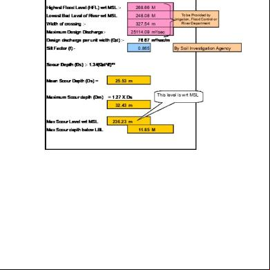
Scour Depth Calculations g2p38
December 2019 37
App. D6 Scour Depth Calculations.doc 3s6i1g
April 2020 26
Scour Depth Calculations-garret's Run Bridge.doc 6w3wh
April 2020 21
Scour Depth Of Retaining Wall Parallel To River 4i5u4w
October 2019 137More Documents from "Perkresht Pawar" k472y
Scour Depth 4p6k23
December 2019 92
Market Segmentation In Banking Sector 2x58
November 2019 75Barringer_ent5_tb_04.doc 2y2p72
December 2019 124
Confederate Pulp And Paper 5g5e20
April 2020 33
Marketing Strategy And Swot Analysis Of Parle G 1g2136
December 2019 168