Micro Drainage Uk Manual 2c1a67
This document was ed by and they confirmed that they have the permission to share it. If you are author or own the copyright of this book, please report to us by using this report form. Report 3b7i
Overview 3e4r5l
& View Micro Drainage Uk Manual as PDF for free.
More details w3441
- Words: 68,001
- Pages: 440
INDUSTRY STANDARD DRAINAGE DESIGN SOFTWARE
SYS1
SIM
SC
MANUAL
CASDeF
FloodFlow
DN
APT
Q OST Qu QuOST
C
MD
P
Micro Drainage
Revision 0 January 2014
®
Micro Drainage® 2014
Examples - introduction
Page 0.1
Working with Micro Drainage® An example led introduction to the Micro Drainage suite.
Page 0.2
Examples - introduction
Contents Introduction, Installation, Help Example 1
System 1 - The Modified Rational Method
Example 2
System 1 - Open Channel Design
Example 3
System 1 - Schedules, Longsections, Plan & 3D Graphics
Example 4
System 1 - Foul Sewer Design with Schedules
Example 5
Source Control - Storage Lake
Example 6
Source Control - Tank Sewer
Example 7
Simulation - Simulation of a drainage system with tank sewers
Example 8
Simulation - Advanced Productivity Tools & CASDeF
Example 9
Channel - The Backwater Step Method
Example 10
Source Control - Infiltration Systems
Example 11
QuOST - Quantities & Costings
Examples - introduction
Example 12
DrawNet (CAD) - Working within AutoCAD®
Example 13
DrawNet - Graphical Model Build
Example 14
FloodFlow - Overland Flow Path Analysis
Example 15
Pluvius – Use of Extended Time Series Rainfall
Appendices Appendix i Appendix ii Appendix iii Appendix iv Appendix v
Hydraulic Conduits IDF, CRP and Hyetograph Rural Discharge Unit Hydrograph Allowable discharge for Example 8
Page 0.3
Page 0.4
Examples - introduction
Introduction
These examples are designed to give you hands-on experience of working with Micro Drainage. They have been created to demonstrate the key features and benefits of the program by addressing most of the common problems encountered in the analysis and design of drainage networks. You should use them in conjunction with the program, referring to the results on-screen where necessary. Images from the program have been used to illustrate the main points of the procedure.
Installing Micro Drainage
With this pack you will have the Micro Drainage installation DVD and a dongle. To install Micro Drainage insert the DVD into the DVD-ROM drive. Do not connect dongle until after the software is installed. Note: Micro Drainage will not run without the dongle - always make sure it is properly in place before trying to run Micro Drainage. If you have Autoplay running, the installation procedure will launch automatically and you will see the Micro Drainage Setup window.
Examples - introduction
Page 0.5
If autoplay is switched off or is not available then proceed as follows: •
From the Start menu select the Run… option.
•
At the Run window type the letter of your DVD-ROM drive followed by :\setup (e.g. d:\setup).
•
Click OK.
At the Setup Window select Install Micro Drainage. The program will display any relevant last minute instructions. When you are happy you are ready to proceed click the Install Micro Drainage button. Follow the on-screen prompts. When the Select Installation Folder window appears, ensure the destination directory is correct.
Click Next to proceed through the Installation wizard.
Page 0.6
Examples - introduction
Upgrade copies
If you are upgrading an existing copy of Micro Drainage, follow the installation procedure as if you were installing a new copy.
Installing a Network copy Windows Server
A License Manager must be installed and running on the server before the software can be installed to the client machines. This can be achieved by selecting the License Manager option from the Autoplay menu, or by running the LMSetup.exe program located in the \Hasp directory on the DVD. The License Manager will require the red dongle to be connected to a free USB port on the server. If you wish to run Micro Drainage on the server then follow the same procedure as above.
Windows Workstations
Follow the same procedure as for a standalone copy.
General Notes
Micro Drainage requires a device driver (haspdinst) to allow communication with the dongle. This is installed automatically by the Setup program. Please ensure this can be accomplished before you begin. The device driver is loaded dynamically (no reboot is required), however this requires you to be logged in as the Windows .
Examples - introduction
Page 0.7
Help
The DVD contains a host of other information relevant to installing and getting started with Micro Drainage. See the What’s New / Help option for the latest installation details or to see the major new features in Micro Drainage 2014.
The topic entitled Read Me contains late breaking information. It is recommended you read this before using the software. The Help system can be accessed from any of the modules by either clicking the Help button (found on most of the dialogue boxes), or by pressing the F1 key. MDHelp provides you with valuable technical data and the detail behind the operation of each module. It follows standard HTML (web page) protocols, with blue text to help you switch between topics. The Contents pane gives you a general overview of the topics covered by Help. However, for a detailed listing of the topics, and to find help quickly on a specific subject, we recommend that you use the Index or Search.
Page 0.8
Examples - introduction
Once you have found the section you want, use the browse buttons at the top of the window to move forwards and backwards through the text. Browse buttons
How Do I
Tutorials are also available for the most commonly asked questions. The tutorials are contained in the last book in the Contents or can be accessed directly from the Help menu in any of the modules.
The problems are listed in two sections, By Module and By Theme. To find the help you require expand the trees.
XP Solutions reserves the right to change any part of the Micro Drainage suite of programs without prior notice. © XP Solutions 2014 XP Solutions recognises all trademarks.
Example 1
Page 1.1
Working with Micro Drainage® Example 1 – System 1 The Modified Rational Method
Page 1.2
Example 1
Introduction
This example takes you step-by-step through a typical network design, using the Modified Rational Method as applied within the System 1 module of Micro Drainage. It has been created to give you hands-on experience of working with Micro Drainage.
Loading Network
Select the Start button and open the Micro Drainage 2014 menu from within the Programs menu:
Click the module you wish to work with. For this example, select Network. This will open all the network build modules held on your licence, and will include System 1. You will now see the Open dialogue box. Click Cancel and we will orientate ourselves with the Micro Drainage package. Select Module Selector from the Window menu and the screen overleaf appears. The Module Selector is the main selection menu of all the Micro Drainage programs. It allows the to change modules or add modules to the current
Example 1
Page 1.3
program. The modules in colour are those currently running. You can add or remove a module by clicking on it. System1, Simulation, DrawNet and QuOST are grouped under Network, but can be run separately. APT, CASDeF and FloodFlow add additional functionality to these modules. Source Control, Channel and Pluvius are separate executables and can be launched from the Module Selector.
If you select a module that is not available on your licence you will be offered the option to start the 30 Day Time Trial. This allows you to try-out all modules that have not been purchased for 30 days. The current active modules are listed in the bottom left-hand corner of the screen. In the Module Selector select the System 1 module so its’ icon is coloured; turn off all other modules by selecting them so they grey out. Menus within the program will update to display all available options for active modules.
Page 1.4
Example 1
The Edit menu presents you with options for the preparation and selection of pipe, manhole, conduit and rainfall libraries which are also available where required within each module. For these functions, see Appendix i and Appendix ii, though you do not need them for this example. The Options menu gives you the choice of industry standard formulae for the hydraulic gradient and flow calculations. You can choose the combination which best suits your requirements, but note that once you have started a project you cannot go back and change your selection for that project. Close the form by selecting the cross. You are now ready to start the first example.
Example 1
Start a New Job
Page 1.5
Reopen the System 1 Open dialogue box by selecting Open from the File menu. Choose the New Storm option by highlighting it and then clicking OK.
Design Criteria
You will now see the Design Criteria screen:
Page 1.6
Example 1
Rainfall Details
Begin by choosing the Rainfall Method. For this example we will accept FSR Rainfall and England & Wales for the Region. In a real project you would select the method and Region by clicking on the arrow to the right of the box. See Appendix iii for more details on how to use an IDF Library.
Note: FEH Rainfall should not be used below 30 minutes duration. This means that until further research is carried out by CEH Wallingford to confirm its use for short durations, it cannot be used for a time of concentration below 30 minutes. In the case of hydrograph methods (Simulation and Source Control) if the 15 minute storm is critical then it should be checked using FSR unless there is further advice from CEH Wallingford. Proceed to enter the remaining Design Criteria as shown on page 1.5. Note: All these values can be entered by clicking on the relevant box or by using the keyboard arrows and then typing.
Pipe and Manhole Sizes
Micro Drainage allows you to specify your own pipe and manhole libraries instead of the Standard libraries shown by default. Simply click on the button next to the Pipes box and the Pipe Sizes form appears.
Example 1
Page 1.7
You may create your own library which can be saved for future use. Or you can load any pipe library saved as a file with the extension .pipx. The same approach is taken to change the manhole sizes. Manhole size library files have the extension .mhsx. Size libraries can also be created and edited from the Edit menu in the Module selector available from the Window menu. Further information is given in the Help. When you have finished entering the data, click OK to proceed.
Creating the network - Network Details
System 1 will now present you with the Network Details spreadsheet.
We will use this spreadsheet to design the following drainage network: 1.000
3.000
1.001
2.000 2.001
1.002
1.003
1.004
The known data for the network are as follows:
Page 1.8
Example 1
Pipe Pipe Fall Slope Area Time Base Pipe no length [m] [1:x] Entry Flow Rough
US/IL [m]
US/CL [m]
Pipe DIA
1.000 100
1.000
100
R
R
1.001 50
R
R
R
2.000 20
0.25
3.000 35.5
R
2.001 21.6
0.25 100
5
10
0.6
0.5 0.01
R
R
R
100
R
R
125
0.02
R
R
R
100
R
R
R
R
R
R
R
1.002 25
R
R
1.52
R
356
1.003 78.9
R
490
5.7
R
2
1.004 100
R
500
R
R
1500
Note: Here, R denotes Return. Where no entry is shown, System 1 will automatically skip the column. This procedure applies within all subsequent examples. Note also that where a pipeline is entered in sequence, you can hit Return instead of entering the next pipe number. Thus for pipe 1.001 you could use the Return key; however, pipe 2.000 breaks the sequence and must be entered manually. We will now proceed to enter each line in turn.
Completing the spreadsheet
Note that the first box of the spreadsheet is automatically highlighted. Enter the data for pipe 1.000 by typing the numbers and pressing Return. Pipe Pipe Fall Slope Area Time Base Pipe US/IL no length [m] [1:x] Entry Flow Rough [m]
US/CL [m]
Pipe DIA
1.000 100
R
R
1.000
0.25
5
10
0.6
100
Note that Slope calculates automatically and that Pipe Diameter calculates when you hit Return for the last time. System 1 will always automatically select the smallest available section from the pipe library you have chosen in this case, the Standard pipe library. In a live project, do not enter a value for Pipe Diameter unless you are sure it is appropriate to do so - for instance if you are working with an existing network.
Example 1
Page 1.9
Upstream Invert Levels, Area and Time of Entry are shown in red, because they are values which you have specified and are not calculated by System 1.
Immediate
Note how the results of your entries are automatically calculated in the lower row. This means that you can see immediately whether or not the values you have used are achieving the desired effect.
Correcting errors
If you are not satisfied with the data in the upper half of your spreadsheet, you can correct any errors simply by highlighting the box concerned. This can be done either with the mouse (by pointing and clicking) or using the keyboard arrows. When the box is highlighted simply key in the correct values. Note: If you do not specify a pipe number or length, System 1 automatically warns you to do so before allowing you to move on.
Pipe 1.001
First, experiment with the error facility by entering 1.002 for Pipe Number. System 1 warns you that it is an Invalid Pipe Number. Enter the correct value, followed by the remainder of this sequence: Pipe Pipe Fall Slope Area Time Base Pipe US/IL US/CL no length [m] [1:x] Entry Flow Rough [m] [m]
Pipe DIA
1.001 50
R
R
100
0.5
R
Notice how Fall automatically calculates when you key in the value for Slope. After you have entered Area, System 1 automatically takes you to US/CL (upstream cover levels), since the program automatically calculates the values in between. We will be entering cover levels later, so here simply hit Return to move to Pipe Diameter. Hitting Return here (or entering 0) automatically calculates the value and moves you to the next row of the spreadsheet. You can alter the automatic calculations if you need to, using the keyboard or
Page 1.10
Example 1
mouse as described previously. However, Time of Entry cannot, of course, be changed as this is only required at the head of a branch line. Equally, you should not specify an upstream invert level (US/IL) unless you wish to specify a backdrop. System 1 automatically places the pipes soffit-tosoffit or invert-to-invert, in accordance with the options chosen in the Design Criteria. Accordingly, the automatically calculated invert level is shown in blue, whereas an invert level which you specified would show as red.
Pipes 2.000 and 3.000
Now enter the following two rows: Pipe Pipe Fall Slope Area Time Base Pipe US/IL US/CL no length [m] [1:x] Entry Flow Rough [m] [m]
Pipe DIA
2.000 20
0.25
3.000 35.5
R
125
0.01
R
R
R
100
R
R
0.02
R
R
R
100
R
R
As both these pipes are at the head of a branch line, the Time of Entry is automatically entered, using your original specified time (5) as a default. Similarly, Pipe Roughness defaults to 0.6; if you alter this value, the new value will then be used as the new default by the program. In this instance, pipes 2.000 and 3.000 have a velocity which is below the recognised minimum of 1m/s as specified by Sewers for Adoption. Accordingly, they are shown in green. Note: Some specifications are less stringent and require 0.7m/s (EN 752). 0.75m/s has been the traditional minimum (formerly 2½ ft/s 2005 1969) used for several decades and can be acceptable to approving authorities where pumping can be avoided by its adoption.
Pipe 2.001
Now enter this row: Pipe Pipe Fall Slope Area Time Base Pipe US/IL no length [m] [1:x] Entry Flow Rough [m]
US/CL [m]
Pipe DIA
Example 1 2.001 21.6
Page 1.11 R
R
R
R
R
Note that Fall, Slope and Diameter are not specified here. This is the only time that the program uses the minimum velocity specified in the Design Criteria. This is what is meant by Auto-Design in the Design Criteria screen. A diameter and slope (or fall) will be chosen by System 1, which will yield a velocity within the specified range. However, note that if a slope or fall is chosen, then the program chooses the smallest diameter, regardless of velocity. Conversely, if a diameter is chosen and not a slope/fall, then the program calculates the minimum slope required to take the flow - again, regardless of velocity. In addition, note that the slope of 2.000 is automatically altered to bring its downstream end level with 3.000, removing a small backdrop. The note at the bottom of the screen tells you that this has been done.
Pipe 1.002
Enter the following row: Pipe Pipe Fall Slope Area Time Base Pipe US/IL no length [m] [1:x] Entry Flow Rough [m]
US/CL [m]
Pipe DIA
1.002 25
R
356
R
R
1.52
Here, you specify the diameter and the 356 appears in red. The slope is given to closely match the flow. As you can see, you can specify non-standard diameters as well as standard diameters.
Pipe 1.003
Enter the following row: Pipe Pipe Fall Slope Area Time Base Pipe US/IL no length [m] [1:x] Entry Flow Rough [m] 1.003 78.9
R
490
5.7
US/CL [m] R
Pipe DIA 2
This time you are specifying both the Diameter and the Slope. It is no mistake that the diameter is 2. When you specify a diameter, which is less than 66 you are in fact specifying a hydraulic section, which is held in an internal library of the most commonly used non-circular sections.
Page 1.12
Example 1
The properties of these sections, which include box culverts, open channels, double and triple pipelines and egg shaped sewers, can be viewed by clicking the Conduits button when you are in the Diameter column of the spreadsheet. In a real project you can also create or load a conduit library of your own. Appendix ii has full details of this facility.
Pipe 1.004
Enter the following row: Pipe Pipe Fall Slope Area Time Base Pipe US/IL no length [m] [1:x] Entry Flow Rough [m]
US/CL [m]
Pipe DIA
1.004 100
R
1500
R
500
R
Here we specify both Slope and Diameter, as you would if the pipe already existed. The 1500mm pipe has spare capacity and the program accepts it. If the pipe was under capacity, System 1 would overrule you and increase the diameter. A way to avoid this automatic upgrading when you are working with an existing system that may be overloaded is explained in a later example.
Checking your entry
Your Network Details spreadsheet should now look like the following example:
Example 1
Page 1.13
Saving your work and opening new projects
Before we examine how to edit data in a completed project, we will save and re-open this finished version. To do so, select Save from the File menu. You will then be presented with the Save Network File window:
In the File name box enter the title Example1 and click Save, or press Return. Note: System 1 is not case-sensitive when searching for file names, so the use of capitals is not essential when opening or re-opening files. To confirm that your file has been saved, exit from System 1 by selecting Exit from the File menu. Now follow the procedure for opening System 1 via the Start button we used at the beginning of this example. When the Open screen appears, the option to continue with Example1.mdx will be displayed. Click on its icon to highlight it and select OK, and you are returned to the Network Details screen. You can open and save files quickly using the toolbar icons: Saves your file Opens a file
Editing
Page 1.14
Example 1
Editing an existing line
Go to pipe 1.001, either by using the scroll bar and clicking on that line or by using the keyboard arrows. Enter a value of 125 for Slope - don't forget to hit Return. System 1 automatically re-calculates the values for pipe 1.001 and all pipes downstream. Note: If you now try to alter the value for Slope again, you will find that the cursor automatically highlights Fall and not Slope. To re-calculate Slope, enter a 0 for Fall and the original value of 100 for Slope. Once again System 1 re-calculates and a value of 0.500 is restored for Fall.
Deleting a pipe
Highlight pipe 1.001. To delete this pipe, click on the Delete Pipe icon in the toolbar. Deletes a pipe The Delete Pipe dialogue box now appears.
The number of the pipe highlighted is automatically shown. However, you can select another pipe number if you prefer. To delete the pipe, simply click OK or press Return. Note: When you delete pipe 1.001, System 1 automatically re-numbers the remaining pipes, e.g. pipe 1.002 is now pipe 1.001, pipe 1.003 is now pipe 1.002 etc.
Example 1
Page 1.15
Inserting a pipe
To insert a pipe, highlight a pipe following the point at which you wish to insert a new pipe. For this example, click on pipe 1.001. Then choose the Insert Pipe icon. Inserts a pipe The Insert Pipe dialogue box now appears. We have two choices. Upstream of… is to insert a pipe which flows into the selected pipe, as would be required here. Downstream of… is to insert a pipe which receives flow from the selected pipe.
You can accept the number of the specified pipe, or select a different pipe from the network. However, for this example click Cancel, because we will shortly restore pipe 1.001 using a different function. If you had clicked OK, System 1 would have inserted a blank row above pipe 1.001 and would again automatically re-number the rest of the spreadsheet.
Re-inserting the deleted pipe – Revision Manager
Selecting Previous Revision from the File menu re-inserts the pipe you deleted. This uses the Revision Manager function which stores a history of data states and edit actions in a database which can be viewed by selecting Revision Manager from the File menu.
Page 1.16
Example 1
The Revision Manager will be operating if Save Undo Information is checked on under the Settings tab. The History tab shows all saved revisions which can be restored by selecting a Revision and clicking Undo.
Longitudinal section
The Longsections function gives you a full graphic representation of the network. To display a longitudinal section, click the Longsections icon. Longsections The screen presents you with a Longitudinal section at the point within the network corresponding to the location of the cursor on the spreadsheet. The default settings only show 1 pipe.
Previous pipes displayed
Above the Longsection itself is a command enabling you to alter the number of pipes displayed on the screen at one time. To increase the number of pipes, click the up arrow. To reduce the number of pipes, click the down arrow. Alternatively type in the box the number of pipes you wish to view and the Longsection will automatically update. You can experiment with this facility by moving the box to the right-hand side of the scroll bar. In our example, there are five different pipes in the
Example 1
Page 1.17
main line; System 1 allows you to view up to thirty pipes at a time. Click the up or down arrow until the command reads 5 or simply type 5 in the box. You will now see all pipes of the main line displayed in longsection. Now click the down arrow, so that the command reads 4. System 1 removes pipe 1.000 and zooms you in closer to the remaining pipes displayed. Change the number of pipes displayed back to 5. Note: If you had clicked the up arrow, the screen would have remained unchanged, since there are only five pipes in this line. There are several icons above the Longsection which we can use to adjust the display. Click the icon below to view the cross-section of each pipe showing the proportional depth and proportional velocity of the flow. Show Cross-section
You can move along the network using the box in the scroll bar beneath the display. Move the box to the right-hand end of the bar to see a full display.
Page 1.18
Example 1
Note: The blue circle for pipe 2.001 is shown above the pipeline profile, to indicate that a backdrop has been incorporated at the junction of the two lines. This is because the invert level for pipe 2.001 (99.716) lies outside the minimum backdrop height of 0.200m specified in Design Criteria. Had it fallen within the specified minimum, System 1 would have automatically recalculated to eliminate the requirement for a backdrop. Branches can be turned on by depressing the Include branch lines option: Include branch lines Branch lines are shown in Blue, to change colours on screen or for printing see Example 3. To view a branch, move the box so that the junction of the branch with the main line is the last section to be displayed on the screen. In this example, move the box approximately to the centre of the scroll bar.
You will now see pipes 2.000 and 2.001, with a blue circle indicating the branch with pipe 3.000 and a pink circle showing where pipe 2.001 s the main network.
Example 1
Page 1.19
Pause?
You have now completed the first stage of Example 1. This is an appropriate place to take a break if you need one.
Managing windows in System 1
A key benefit of Micro Drainage is the facility to move between the elements of each module quickly and easily. Using our example, we will now practice sizing windows and arranging them on the System 1 desktop.
Sizing windows
Use the Windows re-sizing button to shrink the Longsections screen without sending it to the Task Bar.
You should now see a scaled down version of Longsections with the Network Details spreadsheet behind it:
Page 1.20
Example 1
Switching between windows
For this example, you are going to delete a pipe to demonstrate how System 1 automatically re-calculates between functions - and how easy it is to switch between the functions to see the results. First, click on the Design Criteria icon: Design Criteria Design Criteria appears in front of the existing screens. Then choose Cascade from the Window menu and all three Windows are arranged tidily on the screen. Select the Network Details window by clicking in its title bar. You can work with the data within the spreadsheet even though the window does not fill the screen. To make all the title bars visible again, choose Cascade from the Window menu. Before proceeding, make sure you have saved all your work so far. Then delete pipe 1.003, following the procedure set out in Deleting a pipe on page 1.14. Then click on the Longsections title bar and expand the screen by clicking the middle re-sizing button. Adjust the scroll bar until the complete network is shown (by sliding the box to the right-hand side of the scroll) and ensure that the command box at the top of the screen shows 5 Pipes. You will see that in fact only four pipes are displayed, since the original pipe 1.003 has been removed. Pipe 1.004 is the new pipe 1.003, as specified on the Network Details spreadsheet. Finally, choose Cascade again to make all three functions of System 1 visible. Note: A quick way to switch between windows using the keyboard is to hold down Ctrl and use the Tab button to toggle between the windows. Before moving on, reinstate pipe 1.003 by selecting Previous Revision from the File menu.
Example 1
Page 1.21
Note: If you are familiar with the clicking and dragging capabilities of Windows, you may find it easier simply to click in the title bars of the functions and drag them around the desktop, instead of using the Cascade facility.
Auto-refresh
If Longsections was visible when you altered the pipeline details, you may have noticed that the graphic of the network was automatically changed at the same time. System 1 automatically refreshes Longsections whenever a change is made to the spreadsheet. This is a particularly useful function, allowing you to see each pipe in Longsection as it is added to the network.
Optimise
We will now demonstrate the Optimise function, beginning by entering the cover levels for the network we have already designed.
Entry of cover levels
Enter the following data for each pipe in the US/CL[m] column. Simply type in the numbers and press the down arrow. Pipe number 1.000 1.001 2.000 3.000 2.001 1.002 1.003 1.004
US/CL [m] 103 100.5 102 102.5 100.8 100.7 99.2 98
System 1 warns you (in the Warning bar at the foot of the screen) that the data is inconsistent with the depth of 1.2m designated in the Design Criteria. To see the effect this has, look at Longsections. It may help if you turn on the Show pipe bounds which displays the Design Depth. Show pipe bounds
Page 1.22
Example 1
The effect is particularly marked at the conjunction of pipes 2.001 and 1.002. Note the hydraulic grade line (HGL) which is shown in blue.
Next, return to Network Details and go to the Pipe DIA [mm] column. Delete each of the entries shown in red - i.e. all those figures, which you specified, rather than allowing System 1 to calculate them automatically - by entering zero. Hit Return as you delete each figure and System 1 automatically calculates the new pipe diameters. Then simply click Optimise. Optimise The Optimise dialogue box now appears:
Example 1
Page 1.23
You have, of course, already asked System 1 to re-calculate your pipe diameters. Click Yes or press Y. System 1 re-calculates to produce the optimum design depth at 1.2m throughout the entire network. To see the effect, go to Longsection again. Note that 1.004 does not have its ground profile because the downstream cover level is not known at this stage. In addition, you will see that design depth has been set at 1.2m wherever possible. System 1 uses design depth, measured from the connection height to cover level. This can be further observed in the Network Details by looking at the Warnings/Notes box at the bottom of the screen.
Obstructions underground - how to avoid them
In the event that your optimised network encounters an obstruction somewhere along its length, such as an electrical cable or gas pipeline, System 1 allows you to input a different invert level and pipe diameter for the affected point. In this case, let us assume that pipe 1.001 cannot be placed at the level automatically calculated by System 1. Replace the upstream invert level with a value of 98, to allow the pipe to be laid below the service crossing, and the pipe diameter with a value of 450. When the pipe diameter is entered (and Return) both the level and diameter should be in red as they are specified. Optimise will now leave this pipe in place (unless it is too high or has insufficient capacity). Go to Longsections and note that the network once again fails to follow the ground profile at the optimum depth. If you display the pipes downstream you will see that these pipes have also had their depths increased. Return to Network Details and click Optimise, again choosing Yes at the dialogue box. A return to Longsections shows how System 1 optimises the network throughout its entire length, including the pipes downstream of the fixed pipe which are once more at their minimum design depth. This demonstrates System 1's capacity to optimise an entire system around any number of fixed pipes within the network.
Page 1.24
Example 1
Note: As well as fixing pipes in space it is also possible to specify a different required design depth on a pipe by pipe basis. In this instance pipe 1.001 would require a deeper design depth to drop it below the obstruction. An extra column can be switched on in the spreadsheet from Preferences available from the Network Details toolbar to allow this.
Automatic Optimisation
Finally, let us now use the automatic optimisation facility built-in to System 1 to enter two more pipes. Click the Optimise On icon in the toolbar: Optimise On Now key in the following pipe details: Pipe Pipe Fall Slope Area Time Base Pipe US/IL no length [m] [1:x] Entry Flow Rough [m]
US/CL [m]
Pipe DIA
1.005 50
R
R
0.25
96.000
R
1.006 50
R
250
0.25
95.500
R
R
Choose Longsection again and note how System 1 has automatically specified the new pipes to follow the ground profile.
Deg to a Required Outfall
Many new designs require you to connect into a fixed level, whether it is an existing sewer or watercourse. Hitting this required level has always been the bane of the design engineer and deg from the outfall upwards goes against the forward flow design path of the Modified Rational Method. To reverse design is an onerous task to carry out by hand. System 1 allows you to specify the required outfall level in the Outfall Details and Optimise will redesign the system to meet this level. The design we have completed has an outfall level of 93.2m. However the outfall level we require is 94m so we have missed it by 800mm.
Example 1
Page 1.25
Open the Outfall Details by selecting it from the Network menu.
Enter 94 in the Min IL (m) box and then click OK. Before we do the Full Optimise to meet our required outfall we need to turn the Automatic Optimise function off. Click the icon in the toolbar to turn it off. Optimise Off Now click the Full Optimise button and say Yes to the first warning message. A second warning message will appear asking if you would like to raise the outfall invert as it is lower than 94m.
Click Yes to this message and Optimise will redesign the system.
Page 1.26
Example 1
The Network Details show that the Downstream Invert Level for 1.006 has been raised to meet our required outfall invert of 94m.
Note: As the message suggests a minimum invert level can be specified at any point in the system. An extra column can be switched on in the spreadsheet from Preferences to allow this.
In reaching our minimum outfall System 1 has had to break the minimum cover rule of 1.2m in some places. Look at the Longsections to see the effect of this. You will need to increase the number of pipes displayed to 7 to see the entire network.
Example 1
Page 1.27
Network Schematic
This facility allows you to view a graphic model of the network. Click on the Schematic icon: Schematic The schematic is presented showing whichever pipe is highlighted on the pipeline details at the centre of the system. The pipe is shown in red. The number of pipes to display will need to be increased to 6.
The rest of the pipes in any given line are shown in yellow, while branches are shown in blue. Click on any pipe with the right mouse button and select Properties and the properties of the pipe are shown in a popup window. For more information on Properties see Example 13. You can also move through the system by clicking on branches. Try clicking on branch 2; pipes 2.000 and 2.001 are shown, with an arrow to depict the conjunction with the main line:
Page 1.28
Example 1
Printing within System 1
System 1 gives you the option to print a variety of hard copies, based on the values calculated. All the print commands are located under the File menu. A quicker way to open the dialogue box is to click the Print icon in the toolbar: Print When you select Print, System 1 shows you the Print dialogue box:
These options are self-explanatory; you choose the options you would like to print simply by clicking in the appropriate box. Click the Update Preview button to see a print preview. When you are satisfied with the selected options click the printer icon at the top of the dialogue to send the job to the printer. Page Setup… allows you to edit the margins. The printer can be chosen when you click the print icon in the Print window.
XP Solutions Jacobs Well West Street Newbury RG14 1BD Date 04/12/2013 File Example1.mdx XP Solutions
Page 29
Example 1 System 1 The Modified Rational Method Designed by XP Solutions Checked by Network 2013.1.5 STORM SEWER DESIGN by the Modified Rational Method Design Criteria for Storm Pipe Sizes STANDARD Manhole Sizes STANDARD
FSR Rainfall Model - England and Wales Return Period (years) 1 Add Flow / Climate Change (%) 20 M5-60 (mm) 20.000 Minimum Backdrop Height (m) 0.200 Ratio R 0.400 Maximum Backdrop Height (m) 1.500 Maximum Rainfall (mm/hr) 50 Min Design Depth for Optimisation (m) 1.200 Maximum Time of Concentration (mins) 30 Min Vel for Auto Design only (m/s) 1.00 Foul Sewage (l/s/ha) 1.000 Min Slope for Optimisation (1:X) 500 Volumetric Runoff Coeff. 0.750 Designed with Level Soffits
Time Area Diagram for Storm Time Area (mins) (ha)
Time (mins)
0-4 4.200
Area (ha)
4-8 4.263
Time (mins)
Area (ha)
8-12 0.037
Total Area Contributing (ha) = 8.500 Total Pipe Volume (m³) = 183.571
Network Design Table for Storm PN
Length (m)
Fall Slope I.Area T.E. Base k HYD DIA (m) (1:X) (ha) (mins) Flow (l/s) (mm) SECT (mm)
1.000 100.000 2.500 40.0 1.001 50.000 0.125 400.0
0.250 0.500
5.00 0.00
10.0 0.600 0.0 0.600
o o
225 450
2.000
20.000 1.200
16.7
0.010
5.00
0.0 0.600
o
100
3.000
35.500 1.700
20.9
0.020
5.00
0.0 0.600
o
100
2.001
21.600 0.369
58.6
0.000
0.00
0.0 0.600
o
100
1.002 1.003
25.000 0.325 78.900 1.200
76.9 65.8
1.520 5.700
0.00 0.00
0.0 0.600 0.0 0.600
o o
525 750
Network Results Table PN
Rain T.C. (mm/hr) (mins)
US/IL (m)
Σ I.Area Σ Base Foul Add Flow Vel Cap (ha) Flow (l/s) (l/s) (l/s) (m/s) (l/s)
Flow (l/s)
1.000 1.001
50.00 48.01
5.80 101.575 6.63 98.000
0.250 0.750
10.0 10.0
0.3 0.8
8.8 21.7
2.07 1.01
82.5 160.7
52.9 129.9
2.000
50.00
5.18 100.700
0.010
0.0
0.0
0.3
1.90
14.9
1.6
3.000
50.00
5.35 101.200
0.020
0.0
0.0
0.5
1.70
13.3
3.3
2.001
50.00
5.71
99.500
0.030
0.0
0.0
0.8
1.01
7.9
4.9
1.002 1.003
47.44 46.17
6.79 7.17
97.800 97.250
2.300 8.000
10.0 10.0
2.3 8.0
61.6 203.7
©1982-2013 XP Solutions
2.56 553.3 369.4 3.45 1526.2 1222.0
XP Solutions Jacobs Well West Street Newbury RG14 1BD Date 04/12/2013 File Example1.mdx XP Solutions
Page 30
Example 1 System 1 The Modified Rational Method Designed by XP Solutions Checked by Network 2013.1.5 Network Design Table for Storm PN
Length (m)
Fall Slope I.Area T.E. Base k HYD DIA (m) (1:X) (ha) (mins) Flow (l/s) (mm) SECT (mm)
1.004 100.000 1.550 64.5 1.005 50.000 0.100 500.0 1.006 50.000 0.100 500.0
0.000 0.250 0.250
0.00 0.00 0.00
0.0 0.600 0.0 0.600 0.0 0.600
o 750 o 1050 o 1050
Network Results Table PN 1.004 1.005 1.006
Rain T.C. US/IL Σ I.Area Σ Base Foul Add Flow Vel Cap (mm/hr) (mins) (m) (ha) Flow (l/s) (l/s) (l/s) (m/s) (l/s) 44.68 43.11 41.67
7.65 96.050 8.19 94.200 8.74 94.100
8.000 8.250 8.500
10.0 10.0 10.0
8.0 8.3 8.5
203.7 203.7 203.7
3.49 1540.7 1222.0 1.53 1328.5 1222.0 1.53 1328.5 1222.0
Free Flowing Outfall Details for Storm D,L W Outfall Outfall C. Level I. Level Min Pipe Number Name (m) (m) I. Level (mm) (mm) (m) 1.006
0.000
94.000
94.000
©1982-2013 XP Solutions
Flow (l/s)
0
0
Example 2
Page 2.1
Working with Micro Drainage® Example 2 - System 1 Open Channel Design
Page 2.2
Example 2
Introduction
Pipe networks and open channels share many characteristics and it is therefore appropriate to use System 1 for the design of an open channel system. In this example we will examine how a specific conduit library can be created and analysed, using Micro Drainage’s integral conduit design facility. We will also see how a network combining open channels and pipes can be created. The intention here is to keep all water levels below 600mm. However, in order to allow the Simulation module to show overloading when it occurs, we shall define the section to a depth of 1 metre.
Setting up the network
We need only a few sections to demonstrate the principles involved. The following network will be sufficient:
Example 2
Page 2.3
Begin by opening System 1 and select New Storm. Enter the Design Criteria as follows:
Note that we have given the system 15% spare capacity by allowing for 15% additional flow.
Preference
Click OK to call up the Network Details spreadsheet. However, before proceeding to enter any data, we need to add some additional columns to the spreadsheet. This is done by selecting Preferences from the tool bar. Preferences The Preferences dialogue box presents you with a variety of options, which help you tailor the Network Details spreadsheet to suit your requirements.
Page 2.4
Example 2
You can, for example, switch off any columns you are not interested in. Here, however, note that Pipe Roughness and Manning's n (n) are not ticked. Click on n and Pipe Roughness to tick them as shown below. On the Results tab ensure the Proportional Velocity (Pro. Vel m/s) and Proportional Depth (Pro. Depth mm) fields are selected as shown below. Then click OK.
Data entry
For the first line of the spreadsheet, enter the following. Note that since pipe 1.000 is the first pipe in the line, you could use the automatic pipe numbering facility and simply press Return instead of entering the number manually: Pipe Pipe Fall Slope Area Time Base Pipe no length [m] [1:x] Entry Flow Rough
n
US/IL [m]
US/CL [m]
1.000 100
0.012
100
R
0.5
0.25
R
10
R
Pipe DIA COND BUTTON
The command COND BUTTON here means that you should click the Conduits button when the Pipe Diameter field is highlighted. Conduits
Example 2
Page 2.5
This enables you to load or create your preferred conduit library, from which you can select the required sections.
Setting up the Library We are going to specify two different types of conduit, a built in culvert section and a pipe for this system. This will include deg our own section (see Appendix ii for more on this). The Conduit Picker form defaults to the System tab which contains all 65 default conduits supplied with the software. Select the tab; in this part of the form you can create your own bespoke conduits. Select the Edit button and the Conduit Designer form is loaded. Choose the Free option and enter the following data for the first section.
Click on the Channel button and Micro Drainage automatically calculates the areas and wetted perimeter values.
Page 2.6
Example 2
This gives us a standard trapezoidal section. However, note the connection height: 600mm. Although our specified height is 1 metre, to allow for a proper simulation of extreme conditions within Simulation, where pipes are to be connected to the system we need to ensure that the flow does not come in above our prescribed level for normal flows. Note: The Open Section box is ticked to indicate we have created an open section. The next section is one you can create yourself. Highlight the next row on the spreadsheet and choose the Create option. Then select Define. Enter the following data for the section:
Click OK and the section data are entered onto the spreadsheet. You can use the forward slash and backward slash keys to create the Free symbol in the Symbol column. Note, however that the connection height (measured between the pipes invert and the soffit of the upstream pipe) defaults to the height of the section. You will need to alter this from 1 metre to 600mm. Next, we require a U-shaped section. Enter a width of 500mm, a height of 1000mm and a connection height of 600mm. Then choose Free again and click the U Shape button to calculate the variables for the section.
Example 2
Page 2.7
We now have sufficient sections for our demonstration. They will be saved as part of the .mdx file the next time you save. Alternatively, the sections can be saved as Example2.secx and opened for other projects. Select OK for the Conduit Designer form and return to the Conduit Picker form.
Specifying a section
Specify the first section simply by highlighting it and clicking OK. Note that the section is shown by the value -1. This indicates that it is a conduit taken from your own library, rather than the default. See Appendix ii for more details. For pipe 1.001 enter the following: Pipe Pipe Fall Slope Area Time Base Pipe no length [m] [1:x] Entry Flow Rough 1.001 50
0.3
n
US/IL [m]
0.25
US/CL [m]
Pipe DIA
R
R
Hitting Return instructs System 1 to repeat the last value for Pipe diameter; thus section -1 is chosen again.
Adding a branch
We now wish to specify a pipe branch line discharging into the channel. The data are: Pipe Pipe Fall Slope Area Time Base Pipe no length [m] [1:x] Entry Flow Rough 2.000 20
R
50
0.5
R
R
0.6
n
US/IL [m]
US/CL [m]
Pipe DIA
100
R
R
This time, hitting Return gives us a pipe diameter value of 300mm. For the third section in the channel we want to put in a culvert, we can use one of the predefined culverts in the software. We need to add more fields to the spreadsheet to select one.
Page 2.8
Example 2
Select Preferences button on the Network Details tool bar and click on the Input tab. Check the boxes for Section Type, Connection Height (C.Height) and Conduit Symbol and then click OK. Enter the pipe details as shown below: Pipe Pipe Fall Slope Area Time Base Pipe n US/IL Section Type C. Height US/CL Conduit Pipe No. length [m] [1:x] Entry Flow Rough [m] [m] [m] Symbol DIA 1.002 100
R
R
0.5
600 Culvert
R
R
R
We will specify neither Fall nor Slope. In the Section Type field, click on the dropdown menu and select the 600 Culvert, this refers to the height of the culvert in mm. The software chooses the smallest width culvert that can take the flow (900mm) and displays it in the Pipe DIA column. The Help on culverts and other section types can be found by pressing the F1 key. Note: The cursor is automatically moved into the US/CL column when you press Enter in the Area column since this is not the head of a branchline. Step back to the Section Type column and select the required section from the drop down menu. System 1 calculates the minimum slope required for the culvert to accommodate the flow. However, the branch - pipe 2.000 - is now defined with a connection height of 700mm. This gives us a backdrop of 100mm, since we specified a connection height for the conduit sections of 600mm. The backdrop falls within the minimum backdrop height of 200mm specified in Design Criteria. System 1 therefore corrects the slope for pipe 2.000 from 50 to 40. The warning bar at the foot of the spreadsheet notifies you of the change. Switch to Longsections to see the effect of this:
Example 2
Page 2.9
The dotted line indicates the connection height specified (600mm), whereas the solid yellow line depicts the top of the channel at a height of 1 metre. The culvert 1.002 therefore connects at the level of the dotted line, as does the incoming branch 2.000. Note also that the hydraulic grade line (the approximate water level) is below the 600mm connection height.
Calculating flow capacity
Finally, input the data for pipe 1.003: Pipe Pipe Fall Slope Area Time Base Pipe n US/IL Section Type C. Height US/CL Conduit Pipe No. length [m] [1:x] Entry Flow Rough [m] [m] [m] Symbol DIA 1.003 100
0.5
3
0.012
600 Culvert
R
R
R
Note: As with pipe 2.000 you will need to use the cursor keys to step back to the Manning’s n column. You will now be able to enter the required Manning's n. With a substantially increased area, the flow is too great for a culvert of the same size. System 1 therefore increases the width of the culvert to 1200mm.
Page 2.10
Example 2
For this example we will make the final section open. To find a suitable section from our own conduit file, highlight the pipe diameter field again and click the Conduits button. With a flow/capacity ratio of 1.031, which is 3 per cent greater than the capacity of section -3, the section is greyed out since it cannot accommodate the flow. You are left with the choice of the remaining two sections. Section -1 has a ratio suggesting it will probably flow deeper than our prescribed maximum of 600mm. Therefore click on section -2, with its flow/capacity ratio of 0.317, and then click OK. Section -2 is accepted, accommodating the flow of 1021.9 l/s at a depth of 564mm. Note: Even though section -2 appears in its place on the spreadsheet, the calculations to give the values above will not be made until you have hit Return or moved the cursor off the row.
Simulation
While System 1 provides a snapshot of the flows through the system, and ensures the optimum specification for the return period, it does not provide true backwater analysis. For real-time representation of the hydraulic grade lines, this type of system should be analysed within the Simulation module. When you have completed Example 3 (Schedules) and Example 7 (Simulation) of this manual, or if you are already familiar with the Simulation module, you can proceed to generate true hydraulic grade lines for this system using the following steps.
Enter cover levels
Enter a cover level of 102m for all sections and pipes within the network. Then save the file as Example2.mdx.
Example 2
Page 2.11
Schedules
Open the Network menu, select Outfall Details and enter the values as follows:
Click OK. System 1 automatically schedules the network. To view the Schedules, from the Network Details form click on the Schedules button. Schedules
Note: Between open sections there are no manholes. If required a manhole can be added by changing the US Connection type from Junction to Open Manhole and by entering a diameter into the US/MH Diam/Len column. Save the file.
Page 2.12
Example 2
Module Selector Select Module Selector from the Window menu. Click on the Simulation icon to add the module. Menus within the program will update to display all available options for the Simulation module.
Running Simulation
Click OK at the Simulation Criteria and set the program to analyse At Fine time step from the Analyse menu.
Real Time Backwater Analysis
Call up the Longsections. The red line is an envelope of maximum water levels. Now animate the moving water levels as the storm es through the system. The envelope of maximum water levels may be printed through the Plot module and it is a far more detailed analysis than the static levels available through the Modified Rational Method. The network may also be tested for 10, 20, 30 etc. year storms to observe it overloading and flooding. Example 7 is recommended for those who wish to master Simulation.
XP Solutions Jacobs Well West Street Newbury RG14 1BD Date 05/12/2013 File Example2.mdx XP Solutions
Page 13 Example 2 System 1 Open channel Design Designed by XP Solutions Checked by Network 2013.1.7 STORM SEWER DESIGN by the Modified Rational Method Design Criteria for Storm Pipe Sizes STANDARD Manhole Sizes STANDARD
FSR Rainfall Model - England and Wales Return Period (years) 5 Add Flow / Climate Change (%) 15 M5-60 (mm) 20.000 Minimum Backdrop Height (m) 0.200 Ratio R 0.400 Maximum Backdrop Height (m) 1.500 Maximum Rainfall (mm/hr) 100 Min Design Depth for Optimisation (m) 1.200 Maximum Time of Concentration (mins) 30 Min Vel for Auto Design only (m/s) 1.00 Foul Sewage (l/s/ha) 0.000 Min Slope for Optimisation (1:X) 500 Volumetric Runoff Coeff. 0.750 Designed with Level Soffits
Time Area Diagram for Storm Time Area (mins) (ha)
Time (mins)
0-4 3.116
Area (ha)
4-8 1.373
Time (mins)
Area (ha)
8-12 0.011
Total Area Contributing (ha) = 4.500 Total Pipe Volume (m³) = 244.509
Network Design Table for Storm PN
Length (m)
Fall Slope I.Area T.E. Base k (m) (1:X) (ha) (mins) Flow (l/s) (mm)
S1.000 100.000 0.500 200.0 S1.001 50.000 0.300 166.7
0.250 0.250
5.00 0.00
S2.000
40.0
0.500
5.00
0.0 0.600
S1.002 100.000 0.136 735.3 S1.003 100.000 0.500 200.0
0.500 3.000
0.00 0.00
20.000 0.500
10.0 0.0
n
HYD SECT
0.012 0.012
DIA (mm)
\/ \/
-1 -1
o
300
0.0 0.600 600 [] 0.0 0.012 \/
900 -2
Network Results Table PN
Rain T.C. (mm/hr) (mins)
US/IL (m)
Σ I.Area Σ Base Foul Add Flow Vel Cap (ha) Flow (l/s) (l/s) (l/s) (m/s) (l/s)
Flow (l/s)
S1.000 S1.001
85.88 83.80
5.70 100.000 6.02 99.500
0.250 0.500
10.0 10.0
0.0 0.0
10.2 18.5
2.39 1466.8 2.62 1606.8
78.4 142.0
S2.000
89.86
5.13 100.000
0.500
0.0
0.0
18.3
2.49
139.9
S1.002 S1.003
74.62 72.10
7.68 8.22
1.500 4.500
10.0 10.0
0.0 0.0
47.0 133.3
99.200 99.064
©1982-2013 XP Solutions
176.2
1.00 462.0 360.1 3.07 3228.7 1022.1
XP Solutions Jacobs Well West Street Newbury RG14 1BD Date 05/12/2013 File Example2.mdx XP Solutions
Page 14 Example 2 System 1 Open channel Design Designed by XP Solutions Checked by Network 2013.1.7 Conduit Sections for Storm NOTE: Diameters less than 66 refer to section numbers of hydraulic conduits. These conduits are marked by the symbols:- [] box culvert, \/ open channel, oo dual pipe, ooo triple pipe, O egg. Section numbers < 0 are taken from conduit table Section Conduit Major Minor Side Corner 4*Hyd XSect Number Type Dimn. Dimn. Slope Splay Radius Area (m²) (m) (mm) (mm) (Deg) (mm) -1 -2
\/ \/
250 1700
1000 1000
70.0
1.033 0.614 1.508 1.050
Free Flowing Outfall Details for Storm D,L W Outfall Outfall C. Level I. Level Min Pipe Number Name (m) (m) I. Level (mm) (mm) (m) S1.003
S
101.000
98.564
98.000 1800
©1982-2013 XP Solutions
0
Example 3
Page 3.1
Working with Micro Drainage® Example 3 – System1 Schedules, Longsections, Plan & 3D Graphics
Page 3.2
Example 3
Introduction In this example we are going to use the Micro Drainage Schedules module to input manhole data in detail. The data for this example is contained in the file Example3.mdx. This can be found in the \Micro Drainage 2014\Data directory.
Loading Schedules The Schedules module is incorporated in System 1. Open System 1 using your favourite Windows method. As usual, System 1 presents you with the Open options box.
The box gives you the option to select the last file you saved or you can open an existing file. Double click Open Existing File and go to the \Micro Drainage 2014\Data directory and open Example3.mdx. Select the Outfall Details option from the Network menu and enter the outfall details as shown overleaf.
When you have checked that the data are correct click OK and return to the Network Details. Input the data as shown for cover levels.
Example 3
Page 3.3
To see the Schedules spreadsheet click the Schedules button. Schedules Click the Schedules button again to return to the standard Network Details spreadsheet. Input the data as shown for cover levels. Move down the column as you enter the data by using the down keyboard arrow. When complete return to the Schedules table to see the results below.
Schedules automatically assigns a number to each manhole. You will note that the figures in the Depth column are shown in green. This is because the values are less then prescribed cover of 0.9m (values that are twice the prescribed cover will also be displayed in green). Entering the cover levels will rectify this.
Manhole Schedules To view the Manhole Schedule, select Manhole Schedule from the Results menu or click the Manhole Schedule icon on the toolbar if you have added it. Manhole Schedule
Longsections Within Longsections, another key feature of Schedules is demonstrated. Click the Show pipe bounds button. Show pipe bounds
Page 3.4
Example 3
Note the purple and red lines, which delineate the upper and lower boundaries for the network. The upper boundary (in purple) is dictated by the required cover level of 0.900; the lower boundary (in red) is set by the minimum outfall established in Design Criteria - in this case, 95.000m.
Intermediate ground levels Schedules gives you the facility to examine intermediate ground levels, using the GL 1/3 (m) and GL 2/3 (m) columns. To test this resource return to the Schedules Network Details, click on the GL 1/3(m) column for pipe 1.000 and enter a value of 99.500. Enter a value of 100.000 for GL 2/3 (m), a warning appears in the Warning box at the foot of the screen due to you do not having the prescribed cover. This facility is particularly useful in instances where the line crosses an area of uneven cover, such as a ditch. Schedules allows you to enter the data, but warns you of the hazard. To see the effect, go to Longsections.
Example 3
Page 3.5
Changing manhole shapes You can change the shape of the manholes from circular (set as default) to rectangular, by simply specifying the Diameter/Length and Width of the manholes. Click on the US/MH Diam/Len (mm) column for pipe 1.000 and key in 1000 for the length and now click on US/MH Width (mm) column and key in 750 for the Width. The value for the diameter of 1050 (mm) disappears. Schedules shows the values in red, because you have specified them rather than allowing the program to calculate automatically. Note: The manhole diameters are designed in accordance with the specifications in the Manhole size library. The option to Edit/Create a Manhole Size library can be found in the Design Criteria form.
Making the Earth move Within Schedules you have the facility to achieve a 'virtual' shift in the location of true North. This resource is actually designed to make site work easier by eliminating the need for complex Ordnance Survey coordinates and orienting the site around a convenient local point, such as a site base line. Within Example3 we shall use the following coordinates:
Page 3.6
Example 3
Enter these figures by selecting Manhole Coordinates from the Network menu.
Match box When you click OK, you are warned that your coordinates do not match the pipe lengths.
In fact, the downstream Northing for 1.002 should have been 249864.400. Normally the coordinates take precedence in a design. As the warning box says, you can alter the pipe lengths to suit the coordinates. Click Repair Lengths and click OK to the message advising you what has happened. Open the Storm Network Details spreadsheet and you will see that the length of 1.002 has been reduced from 85m to 84.6m - a difference of 0.4m, matching exactly the error in our coordinates. However, in this instance it is the ground that is wrong, not the pipe. Re-open the Manhole Coordinates and enter the correct downstream Northing for pipe 1.002. Click OK and once again select the Repair Lengths option. A look at the Network Details confirms pipe 1.002 now has the correct length.
Example 3
Page 3.7
Oriental setting Next choose Setting Out Information from the Results menu. With the True Coordinates button selected, you can see that the system is actually oriented at a significant angle away from true North; hence the elaborate coordinates.
Clearly, at midnight on a rainswept site, figures of this complexity do not make the site manager's job easier. To redefine the orientation, select Site Location from the Site menu and enter the coordinates for Manhole 1 and set the Orientation to True - in this case, 20 degrees.
Click OK and return to the Setting Out Information. If you now choose the Site Coordinates option, you will see that the orientation is now true North
Page 3.8
Example 3
and that the figures have been greatly simplified; they are all relative to manhole 1.
Example 3
Page 3.9
Network Plan With coordinates in place you can now view a plan view of the network. Click the Plan icon: Plan The plan view of the network allows you to examine manholes and pipes "in situ".
View Options
Drop down the View Options button menu and ensure the Display Manholes and Display Pipe Numbers buttons are depressed.
Page 3.10
Example 3
Right click anywhere on the drawing and select Band Zoom.
Click and hold down the left mouse button and drag the mouse to define a ‘banding’ region. Release the button to Zoom to the region chosen.
The Pan option allows you to move the area you are viewing by dragging it. Alternatively you may also use the Wheel on your mouse to real time zoom. Use Previous and Extents buttons to switch between magnifications.
Example 3
Page 3.11
3D World View A full 3D graphical representation of your network is available in all modules that have the Plan view. Like the Plan the World View is based on manhole coordinates and represents the true state of the world. Pipes without coordinates will have default coordinates applied so they can be drawn on Plan and in 3D. This is indicated on the Plan by the rings around each manhole. If the coordinates and lengths do not match the pipes would be shown as dotted lines. As with the other views right-clicking on a pipe or manhole and selecting Properties will pop-up relevant information. Select 3D World View from the Graphics menu or using the icon on the Plan View tool bar. Display World View The World View will appear showing a full 3D model of the network and ground.
The com on the left gives you the ability to move around the network and zoom into areas. Look around your system using the com and instructions overleaf.
Page 3.12
Example 3
In the upper toolbar there are a number of options allowing you to alter or add to the items displayed.
View Options
Display Pipes / Manholes These buttons switch the pipes and or manholes on and off. Display Sky This switches on a sky background. If switched off the background is left black. Display Branch Indicators A flag is drawn at the first pipe in each branch. The integer part of the pipe is shown in blue on the flag. A flag is also drawn at each outfall position. In this case the branch number is drawn in green.
Example 3
Page 3.13
Ground Style
No Ground switches the ground profile off. The remaining three options change the way the profile is drawn. The Ground may be drawn as Solid, Wireframe or Transparent. The latter option allows the pipes to be seen through the ground. The Ground is coloured from dark green through to light green and then grey as the level increases. Selection Set By selecting this option it is possible to view only those pipes in the current Selection Set. The pipes that are not in the selection set are displayed in a greyed out manner.
Manhole Colours
By default manholes are shown in grey and all outfalls are shown in green. The Cover Level option colour codes the manholes depending on their cover level. The levels associated with each colour can be seen on the Display Settings. The Depth view colours each manhole according to depth. The depths associated with each colour can be seen on the Display Settings. The Connection option displays manholes in red if the connecting pipes are within a pre-determined angle of each other. The angle can be set from Display Settings.
Page 3.14
Example 3
Pipe Colours By default the main line is drawn in yellow and branch lines are displayed in cyan. The Diameter view colours pipes depending on their size (diameter). The diameters associated with each colour can be seen on the Display Settings. Display Settings The Display Setting window shows the various colour settings used in the various graphical displays. Each colour can be defined. Select the Pipes Screen colour and the select a blue from the pallet.
Screen Defaults Select Screen Default to return the Display Settings to the standard colours. Save Saves the current view to disk as a graphic file. Print Open a Print Preview of the World View which can be sent to a printer.
Example 3
Page 3.15
View Tab
Wireframe Pipes / Manholes Pipes and manholes can be drawn as solid or wireframe. Ground Overlay If a background image is available from the Plan it may be merged with or drawn in lieu of the ground profile. Select the On Ground option to merge the image with the existing ground colour. Alternatively select Instead of Ground to replace the standard ground colouring with the map image. Polygon Detail Change the detail level of the drawing elements. Lower levels will increase frame rates on slower machines. This setting only affects solid polygons. Wireframe elements are always drawn at Low detail.
Page 3.16
Example 3
Model Tab
Overlay Detail Specify the size in pixels of the overlay map. Larger values make the image clearer but use more memory and will reduce frame rate. Horizontal Compression The Horizontal compression scales the XY axis of the model to accentuate falls. Scale All Elements With this option switched off only the pipe coordinates are scaled. Pipe and Manhole dimensions are enlarged so they may be easily seen. This should be taken into if pipe clashes are being checked. Switch this option on to show all the elements of the model in true scale (pipes become oval). For most purposes this option can be left switched off. Use TIN Ground Model If a triangulation data set is available you may switch between a full triangulated terrain model and the default ground generated from manhole cover level only. Use Flat Shading By default the terrain model is smooth shaded. Flat shading may be more appropriate if the terrain contains sharp edges (e.g. curbs).
Example 3
Page 3.17
Rebuild Changing options on the Model tab will not automatically modify the model. Click this button to rebuild the model with the new options. + and - Buttons Rebuilds the model but moves the limits of those pipes included. Use + and – to change the limits of the model slightly.
Saving Schedules as text Schedules gives you the option to save your work as text, for use within a word processing package. This is particularly useful for producing high quality proposals and presentations. To do this, simply choose Save ASCII Manhole Schedules from the File menu. The Save ASCII dialogue box appears. Key in the title of your choice and click Save. Note: You cannot open this file from within Micro Drainage. To view your work, use any popular word processing package, e.g. Microsoft Word, WordPerfect, Lotus WordPro etc. Alternatively click on the Schedules spreadsheet with the right mouse button. The Export menu is displayed.
From here you can choose to Print the data, save it as a .csv, .pdf, html or Excel format. This facility is available from all of the results spreadsheets throughout the suite.
Page 3.18
Example 3
Longsection plots We will now examine the use of the output of longsection images. The Longsection module is embedded into System 1, Channel and Simulation. Go to the File menu and select Plot Longsections. The Plot Preview form will open.
The tabs on the left allow you to specify the parameters for the printouts. The Plot Settings tab displays the variables used to batch the pipes for each drawing. It allows you to choose which pipes are to be plotted and whether you want to include branch lines in your selection. You can print the network with the Hydraulic Grade Lines, which will show the Proportional Depth of water in the pipes. The network can also be printed in Normal view (drawn uphill from left to right) or Handed view (downhill from left to right). Note: To change the page orientation, open Page Setup from the File menu and select Landscape under Orientation.
Example 3
Page 3.19
The Plot to Printer tab determines the drawing format. A margin is drawn on each page. The margin is applied around the edge of the page and between the drawings if more than one drawing is plotted per page. The number of drawings high/wide allows you to determine how many drawings across and down the page are to be included in each plot. Pages to Span specify the number of horizontal pages to be used to give the overall plot.
Note: If you make any changes to the setup tabs then you must click Update Preview for the changes to take effect. The Plot to DXF tab lets you print your Longsection to DXF format. Another facility available is the Plot Designer.
Page 3.20
Example 3
The Plot Designer allows you to add data to the drawings. Click the Plot Setup icon in the lower toolbar. Plot Designer The Plot Designer will appear.
To add the data you require just drag it across from the data table to the top or the bottom of the designer and the print preview will automatically update. You can also change the colours. When you have the relevant data displayed you can save your layout for future designs.
XP Solutions Jacobs Well West Street Newbury RG14 1BD Date 11/02/2014 File Example3.mdx XP Solutions
Page 21
Example 3 Schedules / Longsections Plan / 3D Designed by XP Solutions Checked by Network 2014.1 STORM SEWER DESIGN by the Modified Rational Method Design Criteria for Example3 Pipe Sizes STANDARD Manhole Sizes STANDARD
FSR Rainfall Model - England and Wales Return Period (years) 1 Add Flow / Climate Change (%) 0 M5-60 (mm) 20.000 Minimum Backdrop Height (m) 0.200 Ratio R 0.400 Maximum Backdrop Height (m) 1.500 Maximum Rainfall (mm/hr) 5 Min Design Depth for Optimisation (m) 0.900 Maximum Time of Concentration (mins) 30 Min Vel for Auto Design only (m/s) 1.00 Foul Sewage (l/s/ha) 0.000 Min Slope for Optimisation (1:X) 500 Volumetric Runoff Coeff. 0.750 Designed with Level Soffits
Network Design Table for Example3 PN
Length Fall Slope I.Area T.E. Base k HYD DIA (m) (m) (1:X) (ha) (mins) Flow (l/s) (mm) SECT (mm)
1.000 26.000 1.000 1.001 50.000 1.667
26.0 30.0
0.250 0.500
5.00 0.00
10.0 0.600 0.0 0.600
o o
150 225
2.000 20.000 0.250
80.0
0.010
5.00
0.0 0.600
o
100
3.000 35.500 0.473
75.1
0.020
5.00
0.0 0.600
o
100
1.002 85.000 0.850 100.0
0.250
0.00
0.0 0.600
o
300
Network Results Table PN
Rain T.C. (mm/hr) (mins)
US/IL (m)
Σ I.Area Σ Base Foul Add Flow Vel Cap Flow (ha) Flow (l/s) (l/s) (l/s) (m/s) (l/s) (l/s)
1.000 1.001
5.00 5.00
5.22 100.000 5.57 98.925
0.250 0.750
10.0 10.0
0.0 0.0
0.0 0.0
1.98 2.40
35.0 95.3
13.4 20.2
2.000
5.00
5.39 100.000
0.010
0.0
0.0
0.0
0.86
6.8
0.1
3.000
5.00
5.67 100.000
0.020
0.0
0.0
0.0
0.89
7.0
0.3
1.002
5.00
6.57
1.030
10.0
0.0
0.0
1.57 111.1
23.9
97.183
©1982-2014 XP Solutions
XP Solutions Jacobs Well West Street Newbury RG14 1BD Date 11/02/2014 File Example3.mdx XP Solutions
Page 22
Example 3 Schedules / Longsections Plan / 3D Designed by XP Solutions Checked by Network 2014.1 Manhole Schedules for Example3
MH MH Name CL (m)
MH Depth (m)
MH Connection
MH Diam.,L*W (mm)
PN
Pipe Out Invert Diameter Level (m) (mm)
1 101.250 1.250 Open Manhole 1000 x 750 1.000
100.000
150
3 101.240 1.240 Open Manhole
1200 2.000
100.000
100
1200 1.002
97.183
2 101.126 2.201 Open Manhole
1200 1.001
4 102.000 2.000 Open Manhole
1200 3.000
5 101.359 4.176 Open Manhole
6
98.500 2.167 Open Manhole
1500
98.925
100.000
OUTFALL
©1982-2014 XP Solutions
PN
225 1.000
Pipes In Invert Diameter Backdrop Level (m) (mm) (mm)
99.000
150
300 1.001
97.258
225
3.000
99.527
100
100
2.000
1.002
99.750 96.333
100 300
2367 2144
XP Solutions Jacobs Well West Street Newbury RG14 1BD Date 11/02/2014 File Example3.mdx XP Solutions
Page 23
Example 3 Schedules / Longsections Plan / 3D Designed by XP Solutions Checked by Network 2014.1 PIPELINE SCHEDULES for Example3 Upstream Manhole
PN
Hyd Diam MH C.Level I.Level D.Depth Sect (mm) Name (m) (m) (m)
MH Connection
MH DIAM., L*W (mm)
1.000 1.001
o o
150 225
1 101.250 100.000 2 101.126 98.925
1.100 Open Manhole 1.976 Open Manhole
1000 x 750 1200
2.000
o
100
3 101.240 100.000
1.140 Open Manhole
1200
3.000
o
100
4 102.000 100.000
1.900 Open Manhole
1200
1.002
o
300
5 101.359
3.876 Open Manhole
1200
97.183
Downstream Manhole PN
Length Slope MH C.Level I.Level D.Depth (m) (1:X) Name (m) (m) (m)
MH Connection
MH DIAM., L*W (mm)
1.000 26.000 1.001 50.000
26.0 30.0
2 101.126 5 101.359
99.000 97.258
1.976 Open Manhole 3.876 Open Manhole
1200 1200
2.000 20.000
80.0
5 101.359
99.750
1.509 Open Manhole
1200
3.000 35.500
75.1
5 101.359
99.527
1.732 Open Manhole
1200
6
96.333
1.867 Open Manhole
1500
1.002 85.000 100.0
98.500
©1982-2014 XP Solutions
XP Solutions Jacobs Well West Street Newbury RG14 1BD Date 11/02/2014 File Example3.mdx XP Solutions
Example 3 Schedules / Longsections Plan / 3D Designed by XP Solutions Checked by Network 2014.1 Setting Out Information - True Coordinates (Example3) PN
USMH Dia/Len Width US Easting US Northing Layout Name (mm) (mm) (m) (m) (North)
1.000
1
1000
750 557102.000
249708.000
1.001
2
1200
557110.900
249732.400
2.000
3
1200
557108.000
249779.400
3.000
4
1200
557161.400
249767.200
1.002
5
1200
557128.000
249779.400
PN 1.002
DSMH Dia/Len Width DS Easting DS Northing Layout Name (mm) (mm) (m) (m) (North) 6
1500
557128.000
249864.400
©1982-2014 XP Solutions
Page 24
XP Solutions Jacobs Well West Street Newbury RG14 1BD Date 11/02/2014 File Example3.mdx XP Solutions
Page 25
Example 3 Schedules / Longsections Plan / 3D Designed by XP Solutions Checked by Network 2014.1 Setting Out Information - Site Coordinates (Example3) PN
USMH Dia/Len Width US Easting US Northing Layout Name (mm) (mm) (m) (m) (North)
1.000
1
1000
1.001
2
2.000
0.000
0.000
1200
0.018
25.972
3
1200
-18.782
69.146
3.000
4
1200
35.570
75.946
1.002
5
1200
0.012
75.987
PN 1.002
750
DSMH Dia/Len Width DS Easting DS Northing Layout Name (mm) (mm) (m) (m) (North) 6
1500
-29.060
155.860
Free Flowing Outfall Details for Example3 D,L W Outfall Outfall C. Level I. Level Min Pipe Number Name (m) (m) I. Level (mm) (mm) (m) 1.002
6
98.500
96.333
95.000 1500
©1982-2014 XP Solutions
0
XP Solutions Jacobs Well West Street Newbury RG14 1BD Date 11/02/2014 File Example3.mdx XP Solutions
Page 26
Example 3 Schedules / Longsections Plan / 3D Designed by XP Solutions Checked by Network 2014.1
MH Name
5
1
2
Hor Scale 1200 Ver Scale 250
Length (m)
50.000
100.000 101.250
Invert Level (m)
MH Name
98.925 101.126 99.000 100.000
101.359 97.258
Cover Level (m)
1.000 150 26.0
1.001 225 30.0
99.500
Datum (m)92.000 PN Dia (mm) Slope (1:X)
26.000
6
5
Hor Scale 1200 Ver Scale 250
Datum (m)91.000 PN Dia (mm) Slope (1:X)
Length (m)
98.500
97.183 101.359
Invert Level (m)
96.333
Cover Level (m)
1.002 300 100.0
85.000
©1982-2014 XP Solutions
Example 4
Page 4.1
Working with Micro Drainage® Example 4 – System1 Foul Sewer Design with Schedules
Page 4.2
Example 4
Introduction
This example details the design of a complete foul sewer network with schedules using both the Main Drainage and Fixture Unit methods. This Micro Drainage resource also aids the drafting and production of contract documents. Open System 1 and at the Open screen select New Foul Main Drainage.
Design Criteria
The Design Criteria window appears with default values set to produce the design flows required for gravity sewers on residential developments of 4000 l/unit dwelling/24 hours in accordance with Sewers for Adoption.
Enter the additional data as shown and click OK.
Example 4
Page 4.3
Pipeline Details
The Foul Network Details spreadsheet now appears. Enter the data for the following network: Pipe Pipe Fall Slope Area Houses no length [m] [m]
Base Pipe US/IL Flow Rough [m]
US/CL [m]
1.000 26
R
80
R
58
5
101.100 R
R
25
R
75
R
26
2.000 89
R
45
R
15
R
54
R
50
R
22
3.000 25
R
25
R
36
1.002 52
R
75
R
29
R
R
75
3.2
54
1.500
100
Pipe DIA
101.200 R R
R
100
101.250 R 100.925 R
R
R
100
101.145 R 100.525 R 97.500
R
Here pipes 1.000 to 1.002 serve a housing development. Pipe 1.003 serves an industrial development. Therefore, the industrial flow has been specified in litres/second/hectare and the domestic flow has been input in of the number of houses contributing. It is assumed you have to meet an existing system which is at 95m AOD. In order to make sure our outfall hits 95m, select Outfall Details from the Network menu, enter the following additional data and click OK.
Click Full Optimise to improve the design and save your work as Example4.
Page 4.4
Example 4
Optimise has re-designed the network to produce the optimum cover at 0.9m throughout the network and also a minimum Full Bore Velocity of 0.75 m/sec for each pipe. To provide a self-cleansing regime within foul gravity sewers, the minimum flow velocity should be 0.75 m/sec at one third design flow. Optimise has the ability to re-design the network so that it achieves 0.75 m/sec at one third design flow. Select the optimise to P.Vel at 1/3 Flow option on the toolbar as shown below.
Then click the Full Optimise button.
Example 4
Page 4.5
The results table shows that the minimum of 0.75 m/sec hasn't been achieved in all cases. Pipes 1.000, 2.000, 2.001 and 3.000 all have a Proportional Velocity of less than 0.75 m/sec at 1/3 design flow. Pipe 1.000 is a 150mm pipe with 58 connections (houses). It has been laid at a slope of 1:150 in accordance with Sewers for Adoption. Pipes 2.000 and 2.001 are 100mm pipes with more than 10 connections. They have been laid at a slope of 1:80 in accordance with BS EN 752. Pipe 3.000 is also a 100mm pipe with more than 10 connections and is also subject to the minimum slope (1:80) requirements of BS EN 752. Optimise has increased the slope for this pipe to 1:40.3 to maintain 0.9m cover. Optimise has combined minimum velocity rules, minimum slope recommendations and minimum cover requirements to produce an acceptable design. Note: See also Help – System 1 – Optimise Click Save to save the new design.
Page 4.6
Example 4
Schedules Select Manhole Schedule from the Results menu. System 1 has automatically designed manhole sizes in accordance with the specification set in the Manhole Size library.
A look at Longsections will show you that the network has been designed satisfactorily. You should now have a complete drainage design ready for the production of contract documents.
Discharge Unit Methods A second version of Foul can be accessed within System 1 that allows a network to be designed by specifying a number of discharge units in lieu of houses. Both the BS 8301 and EN 752 methodologies are ed. From the Site menu select the Network Manager option and change the Network Type to Foul – Unit as shown below. Rename the network Foul – Unit in the Name column and then close the form.
Example 4
Page 4.7
At the Design Criteria form select the BS 8301 option and make sure all the other data is as shown.
Click OK to the Design Criteria and the Network Details will appear. The houses entered for the Main Drainage method have been converted to units at a rate of 14 units per house. Change optimse to P.Vel at 1/3 Flow again and click Optimise to re-design the network.
Page 4.8
Example 4
On inspection the results show that the Fixture Unit method produces different results to the Main Drainage method. The Fixture Unit method is more applicable to smaller sites (less than 300 houses) whilst the Main Drainage is more applicable to larger sites. The Fixture Unit method should also be used on sites where there is a mixture of commercial, industrial and residential properties. Finally we will demonstrate how the EN 752 method can be used. Select Design Criteria from the Network menu. Change the Unit Calculation Method to be used to EN 752 and set the Frequency Factor (EN 752 Only) to 0.5. This is a typical frequency factor to be used for dwellings as stated in table C.1 (BS EN 752). Click OK to the Design Criteria and the Network Details will appear. Upon examining the results you will see that no conversion from houses to units has occurred when using the EN 752 method. For this site there are roughly 12 units per dwelling based on the typical values of discharge units (DU) in table C.2 (BS EN 752).
Example 4
Page 4.9
Enter the Units for each pipe as shown below.
Click the Full Optimise button to optimise the network to proportional velocity at 1/3 design flow.
The Results now show the system re-designed to achieve proportional velocity at 1/3 design flow. Where this cannot be achieved the minimum slope recommendations and minimum cover requirements have been applied to produce an acceptable design. On sites where there is a mixture of commercial, industrial and residential properties a Frequency Factor (kDU) can be applied per pipe in accordance with Table C.1 (BS EN 752).
Page 4.10
Example 4
To specify a Frequency Factor per pipe select Preferences from the toolbar. Go to the Input tab and tick the Freq Factor option.
Click OK and the network details will now show an additional column allowing a Frequency Factor (kDU) to be set per pipe.
Printing
This follows the same procedure as the previous example.
Example 4
Page 4.11
Combining Storm and Foul flows
Micro Drainage gives you the facility to analyse simultaneous Storm and Foul flows through a network. To do this, select Network Manager from the Site menu. Test Combined Sewer can be selected from the Toolbar. A copy of the existing network is created as a Storm network or vice versa if a Storm network that you are copying. You are then prompted to enter the Design Criteria for your Storm or Foul flow. Clicking OK presents you with a Network Details spreadsheet, which analyses the dry weather flow condition. Note: In fact, a combined system would usually be analysed first within the System 1 module as a Storm file. You can enter the Foul flow in the Design Criteria window; it is specified in litres/second/hectare. Although this figure is only an approximation, it is suitable for combined analysis since it represents only a small percentage of the total flow. For more detailed analysis of dry weather flow in particular, you can then transfer the data to Foul as described above. This enables you to specify the foul sewage in greater detail and to observe the proportional velocities of flow through the system when it is not raining.
XP Solutions Jacobs Well West Street Newbury RG14 1BD Date 26/02/2014 File Example4.mdx XP Solutions
Page 12 Example 4 System 1 - Foul Sewer Design with Schedules Designed by XP Solutions Checked by Network 2014.1 FOUL SEWERAGE DESIGN Design Criteria for Foul - Main Pipe Sizes STANDARD Manhole Sizes STANDARD
Industrial Flow (l/s/ha) 1.00 Add Flow / Climate Change (%) 20 Industrial Peak Flow Factor 3.00 Minimum Backdrop Height (m) 0.200 Flow Per Person (l/per/day) 222.00 Maximum Backdrop Height (m) 1.500 Persons per House 3.00 Min Design Depth for Optimisation (m) 0.900 Domestic (l/s/ha) 0.00 Min Vel for Auto Design only (m/s) 0.75 Domestic Peak Flow Factor 6.00 Min Slope for Optimisation (1:X) 500 Designed with Level Soffits
Network Design Table for Foul - Main PN
Length Fall Slope Area Houses Base k HYD DIA (m) (m) (1:X) (ha) Flow (l/s) (mm) SECT (mm)
1.000 26.000 0.173 150.0 0.000 1.001 25.000 0.402 62.2 0.000
58 26
5.0 1.500 0.0 1.500
o o
150 150
2.000 89.000 1.113 2.001 54.000 0.675
80.0 0.000 80.0 0.000
15 22
0.0 1.500 0.0 1.500
o o
100 100
3.000 25.000 0.620
40.3 0.000
36
0.0 1.500
o
100
1.002 52.000 1.963 26.5 0.000 1.003 54.000 0.500 108.0 3.200
29 0
0.0 1.500 0.0 1.500
o o
150 225
Network Results Table PN
US/IL (m)
Σ Area Σ Base Σ Hse Add Flow P.Dep P.Vel Vel Cap Flow (ha) Flow (l/s) (l/s) (mm) (m/s) (m/s) (l/s) (l/s)
1.000 100.050 1.001 99.877
0.000 0.000
5.0 5.0
58 84
1.5 1.8
95 79
0.78 1.13
0.71 1.11
12.6 19.6
9.2 10.7
2.000 100.250 2.001 99.138
0.000 0.000
0.0 0.0
15 37
0.1 0.3
26 41
0.52 0.68
0.74 0.74
5.8 5.8
0.8 2.1
3.000 100.145
0.000
0.0
36
0.3
34
0.86
1.05
8.2
2.0
1.002 1.003
0.000 3.200
5.0 5.0
186 186
2.7 4.6
79 130
1.74 1.17
1.71 1.10
30.2 43.9
16.3 27.8
98.413 96.375
©1982-2014 XP Solutions
XP Solutions Jacobs Well West Street Newbury RG14 1BD Date 26/02/2014 File Example4.mdx XP Solutions
Page 13 Example 4 System 1 - Foul Sewer Design with Schedules Designed by XP Solutions Checked by Network 2014.1 Manhole Schedules for Foul - Main
MH MH Name CL (m)
MH Depth (m)
MH Connection
MH Diam.,L*W (mm)
PN
Pipe Out Invert Diameter Level (m) (mm)
1 101.100 1.050 Open Manhole
1200 1.000
100.050
2 101.200 1.323 Open Manhole
1200 1.001
99.877
3 101.250 1.000 Open Manhole
1200 2.000
100.250
4 100.925 1.787 Open Manhole
1200 2.001
99.138
5 101.145 1.000 Open Manhole
1200 3.000
100.145
6 100.525 2.113 Open Manhole
1200 1.002
98.413
7
97.500 1.125 Open Manhole
1200 1.003
8
97.000 1.125 Open Manhole
1200
PN
Pipes In Invert Diameter Backdrop Level (m) (mm) (mm)
150 150 1.000
99.877
150
99.138
100
150 1.001
99.475
150
2.001
98.463
100
100 100 2.000 100
3.000
99.525
100
96.375
225 1.002
96.450
150
OUTFALL
1.003
95.875
225
©1982-2014 XP Solutions
1063 1063
XP Solutions Jacobs Well West Street Newbury RG14 1BD Date 26/02/2014 File Example4.mdx XP Solutions
Page 14 Example 4 System 1 - Foul Sewer Design with Schedules Designed by XP Solutions Checked by Network 2014.1 PIPELINE SCHEDULES for Foul - Main Upstream Manhole
PN
Hyd Diam MH C.Level I.Level D.Depth Sect (mm) Name (m) (m) (m)
MH Connection
MH DIAM., L*W (mm)
1.000 1.001
o o
150 150
1 101.100 100.050 2 101.200 99.877
0.900 Open Manhole 1.173 Open Manhole
1200 1200
2.000 2.001
o o
100 100
3 101.250 100.250 4 100.925 99.138
0.900 Open Manhole 1.687 Open Manhole
1200 1200
3.000
o
100
5 101.145 100.145
0.900 Open Manhole
1200
1.002 1.003
o o
150 225
6 100.525 7 97.500
1.963 Open Manhole 0.900 Open Manhole
1200 1200
98.413 96.375
Downstream Manhole PN
Length Slope MH C.Level I.Level D.Depth (m) (1:X) Name (m) (m) (m)
MH Connection
MH DIAM., L*W (mm)
1.000 26.000 150.0 1.001 25.000 62.2
2 101.200 6 100.525
99.877 99.475
1.173 Open Manhole 0.900 Open Manhole
1200 1200
2.000 89.000 2.001 54.000
80.0 80.0
4 100.925 6 100.525
99.138 98.463
1.687 Open Manhole 1.963 Open Manhole
1200 1200
3.000 25.000
40.3
6 100.525
99.525
0.900 Open Manhole
1200
7 8
96.450 95.875
0.900 Open Manhole 0.900 Open Manhole
1200 1200
1.002 52.000 26.5 1.003 54.000 108.0
97.500 97.000
Free Flowing Outfall Details for Foul - Main D,L W Outfall Outfall C. Level I. Level Min Pipe Number Name (m) (m) I. Level (mm) (mm) (m) 1.003
8
97.000
95.875
95.000 1200
©1982-2014 XP Solutions
0
XP Solutions Jacobs Well West Street Newbury RG14 1BD Date 23/12/2013 File Example4.mdx XP Solutions MH Name
Page 15
Example 4 System 1 - Foul Sewer Design with Schedules Designed by XP Solutions Checked by Network 2013.1.7 F8
F7
F6
F1
F2
Hor Scale 2500 Ver Scale 250
54.000 F6
52.000
99.975 101.100
F1.001F1.000 225 225 65.5 134.6 99.782 101.200 99.782
97.500
97.000
Length (m) MH Name
F1.002 225 18.7
96.300 96.375
Invert Level (m)
95.800
Cover Level (m)
F1.003 300 108.0
99.159 100.525 99.400
Datum (m)91.000 PN Dia (mm) Slope (1:X)
25.00026.000
F4
F3
Hor Scale 2500 Ver Scale 250
Length (m)
F2.000 150 150.0 99.607 100.925 99.607
99.234
Invert Level (m)
100.525
Cover Level (m)
F2.001 150 145.0
54.000
100.200 101.250
Datum (m)93.000 PN Dia (mm) Slope (1:X)
89.000
©1982-2013 XP Solutions
XP Solutions Jacobs Well West Street Newbury RG14 1BD Date 23/12/2013 File Example4.mdx XP Solutions MH Name
Example 4 System 1 - Foul Sewer Design with Schedules Designed by XP Solutions Checked by Network 2013.1.7 F6
F5
Hor Scale 2500 Ver Scale 250
100.095 101.145
Invert Level (m)
99.475
Cover Level (m)
F3.000 150 40.3 100.525
Datum (m)92.000 PN Dia (mm) Slope (1:X)
Length (m)
25.000
©1982-2013 XP Solutions
Page 16
Example 5
Page 5.1
Working with Micro Drainage® Example 5 - Source Control Design of a storm water storage lake
Page 5.2
Example 5
Introduction
In this example we are going to work with the Source Control module to design a tank/pond to serve as a landscaping water feature.
Design criteria •
The tank/pond shall provide sufficient storage to limit the run-off from a 26.9ha (paved area) site to 1300 l/s during a storm of a 100 year return period for both summer and winter storms.
•
No drainage point (or top of embankments) is to be lower than 500mm above the 100 year storm top water level.
•
The overflow should be capable of ing a storm of a 1000 year return period without the water level rising to within 200mm of the top of the embankment.
The following picture shows a permanent water feature with 1.5m available for storage:
Loading Source Control
Follow your preferred procedure for opening Source Control. Before proceeding with a design it is useful to obtain an estimate of the storage requirements in order to establish the parameters within which we will be working. Therefore at the Source Control Open screen, choose Quick Storage Estimate.
Example 5
Page 5.3
Quick Storage Estimate
Enter the data as shown in the example below - some of the figures are default values. When you are satisfied that the data are correct, click Analyse.
Source Control tells you that it is performing full routing calculations. The following information box gives you the results:
Make a note of these parameters and click OK. The Global Variables appear to begin a more detailed design.
Page 5.4
Example 5
Global Variables
Check that the options shown match the entries shown on the example below. If they do not, you can select them by using the mouse and clicking on the arrows at the side of each box, or by using Tab and the keyboard arrows.
Rainfall & Network Details
Click OK and Source Control opens the Rainfall & Network Details form:
We are going to run both Summer and Winter storms so make sure they are both selected. Note: The Cv value for winter is higher than for summer as UCWI is on average 50mm higher in winter.
Example 5
Page 5.5
The program assumes no upstream network unless a Storage Volume is entered. If a storage volume is entered the other details can be entered which the software uses to calculate the relationship between discharge and proportional cross sectional area which may affect the Inflow Hydrograph if there is significant upstream storage. Enter the data as shown on the previous page - again using Tab and the arrows or the mouse, according to your preference - and click OK.
Time Area Diagram
Your next screen will be the Time Area Diagram spreadsheet. Enter the data as shown in the right-hand column. To do this, simply highlight each box by clicking or using the keyboard arrows and then keying in the value. Then click OK.
Note: In a real project, Time/Area details saved in the System1 module (for storm networks) under the File menu may be loaded into the above spreadsheet. Click the Import button to search for files with the .tadx or .tad extension.
Page 5.6
Example 5
Plan Area of Pond
Next you will see the Tank or Pond dialogue box:
After entering the Cover Level and Invert Level you can select the depth increment required or type in only the heights at which the shape of the pond changes. For this example click 0.1 button to set the depth increment at 0.1m. You can enter the Area at each depth increment using the Repeat button as required. However, for this example, enter 4250m² at depth 0.0m. Click the calculator button and the Shape Calculator form appears. We will use this to set the Side Slope at 1:4. We could also use the calculator to set the volume.
Note: Shape Calculator will set the side slope or volume for the entire depth if one cell is selected or the highlighted section if more than one cell is selected.
Example 5
Page 5.7
If we click on each area cell the available volume is displayed in the bottom left hand corner, for 1.5 m depth this is within our Quick Storage Estimate range. When you are satisfied the data are correct, click OK.
Note: Scale Factor enables you to adjust the values of the data without reentering the entire array. Simply enter the increment by which you wish to increase or decrease the values and click Scale.
Setting Parameters
Source Control next moves to the Weir Outflow Control dialogue box. We will use the Calculator to size the weir based on the required outflow so click the Calculator icon and enter the details as shown.
Page 5.8
Example 5
A weir width of 415mm is suggested. Click Apply to accept this size, enter the other weir values as shown below and click OK.
Repeat this procedure with the Weir Overflow Control dialogue box.
Click OK and then hit the Go button in the toolbar. Run Analysis The drop down arrow allows you to choose the increment at which to analyse the structure. The default is the finest increment.
Example 5
Summary of Results
Page 5.9
Source Control performs the final routing calculations, presenting you with a request to save the data. Click Yes and save the data as Example5. At the conclusion of the Save procedure Source Control presents you with the summary of results for the 100 year return period for both summer and winter storms:
Page 5.10
Example 5
Full routing tables
To view a detailed result, click the Hydrograph Tables icon in the toolbar. Hydrograph Tables Source Control opens the Hydrograph Tables, beginning with a Winter storm of 120 minutes duration as this is the critical storm. Use the scroll bar to the right of the table to view the effects of the storm in its entirety. The Storm Selector allows the summer/winter analysis of any of the storm durations to be viewed.
Example 5
Page 5.11
Graphs
Next, select the Graphs icon. Graphs Source Control displays the Graphs screen.
Once again, you can choose to view either summer or winter and you can change the storm duration using the Storm Selector. You will note also that Source Control presents you with several options for viewing the graphs themselves. Select these simply by clicking on each graph icon on the Graph toolbar – turn on all the options to see the layout above. Note - window management: For easy switching between results windows, you can use the Tile or Cascade commands under the Window menu. As set out in Example 1, you can re-size the windows according to preference.
Page 5.12
Example 5
Animation
Source Control allows you view your results in the form of an animated simulation of a storm. To experiment with this, click on the Animation icon. Animation A Video Controls box appears which features icons that replicate the functions of a standard media player. Click Play.
The Animation also gives you the option to view either summer or winter storms. Select 120 min Winter from the Storm Selector. The drawing features a red disk, which signifies the critical level for the design. An animated blue disk indicates the level during the course of the storm. To view the Trace option, ensure the button is depressed and press Play again, you will see the level animated in pale blue, giving you a time elapsed picture of the storm.
Example 5
Page 5.13
Press Play again and pause the storm when the timer reaches 76 minutes. You can now use the Forward and Rewind buttons to watch the flow minute-byminute. To re-start the animation at any point, simply press Stop, followed by Play.
Printing
To print, hit the Print icon. Print The Print dialogue box appears.
These options are self-explanatory; you choose the options you would like to print by clicking in the appropriate box. Click the Update Preview button to see a print preview. When you are satisfied with the selected options click the printer icon at the top of the form to send the job to the printer.
Page 5.14
Example 5
Testing overflows
Before proceeding to look at the results in detail, it is appropriate now to test the overflow for capacity. Close all the results forms down except the Summary of Results. The Window menu will help you to identify forms that are still open. From Table 7.2. Ciria Book 14 (based on ''Floods and reservoir safety, an engineering guide, Institution of Civil Engineers'') let us assume that a breach of the reservoir will pose negligible risk to life and cause limited damage. This will require the overflow to be tested for a 1000 year return period (annual probability of 0.1%). Select Rainfall Details from the Edit menu. Source Control returns you to the Rainfall and Network Details dialogue box. Change the return period from 100 to 1000 years and click OK. You will notice that as soon as you have clicked OK the software will reanalyse the data and update the Summary of Results. This is because the default settings in Preferences are set to Maintain Results. If you prefer to use the Go button to run the analysis you can select the Preferences from the File menu and change the Analysis to . Click the Save icon to save the file as Example5. Source Control will automatically replace the old example with the new. You will note that the summary of results shows a maximum depth of 1.786m, which is still within our 1.8m limit (i.e. 200mm below the embankment) but the Status column is displaying Flood Risk. The margin for Flood Risk warning can also be edited via Preferences. that this is a test only for the capacity of the overflow; if it were inadequate we would increase the length, not the storage.
XP Solutions Jacobs Well West Street Newbury RG14 1BD Date 02/01/2014 File Example5.srcx XP Solutions
Page 15
Example 5 Source Control Storm Water Storage Lake Designed by XP Solutions Checked by Source Control 2014.0 (Beta 2) Summary of Results for 100 year Return Period Storm Event
15 30 60 120 180 240 360 480 600 720 960 1440 2160 2880 4320 5760 7200 8640 10080 15 30 60 120 180 240 360 480
min min min min min min min min min min min min min min min min min min min min min min min min min min min
Max Level (m)
Summer Summer Summer Summer Summer Summer Summer Summer Summer Summer Summer Summer Summer Summer Summer Summer Summer Summer Summer Winter Winter Winter Winter Winter Winter Winter Winter Storm Event
15 30 60 120 180 240 360 480 600 720 960 1440 2160 2880 4320 5760 7200 8640 10080 15 30 60 120 180 240 360 480
min min min min min min min min min min min min min min min min min min min min min min min min min min min
Status Max Max Max Max Max Depth Control Overflow Σ Outflow Volume (m³) (l/s) (l/s) (l/s) (m)
100.937 0.937 641.1 0.0 641.1 4399.9 101.151 1.151 872.9 0.0 872.9 5528.4 101.290 1.290 1035.7 0.0 1035.7 6285.7 101.349 1.349 1108.2 0.0 1108.2 6616.2 101.346 1.346 1103.9 0.0 1103.9 6596.2 101.320 1.320 1072.1 0.0 1072.1 6453.5 101.255 1.255 994.4 0.0 994.4 6096.1 101.191 1.191 919.4 0.0 919.4 5748.1 101.133 1.133 852.5 0.0 852.5 5432.6 101.081 1.081 794.5 0.0 794.5 5154.0 100.993 0.993 699.4 0.0 699.4 4691.5 100.864 0.864 567.6 0.0 567.6 4027.6 100.737 0.737 447.6 0.0 447.6 3391.1 100.652 0.652 372.5 0.0 372.5 2973.4 100.542 0.542 282.3 0.0 282.3 2442.5 100.473 0.473 229.8 0.0 229.8 2113.1 100.424 0.424 195.1 0.0 195.1 1885.6 100.387 0.387 170.1 0.0 170.1 1714.5 100.358 0.358 151.3 0.0 151.3 1579.9 101.031 1.031 740.5 0.0 740.5 4893.4 101.249 1.249 986.7 0.0 986.7 6061.3 101.420 1.420 1196.2 0.0 1196.2 7012.7 101.460 1.460 1247.1 0.0 1247.1 7242.3 101.429 1.429 1208.2 0.0 1208.2 7068.8 101.379 1.379 1144.7 0.0 1144.7 6781.6 101.275 1.275 1018.3 0.0 1018.3 6206.5 101.185 1.185 911.8 0.0 911.8 5710.6 Rain Flooded Discharge Overflow Time-Peak (mins) Volume Volume (mm/hr) Volume (m³) (m³) (m³)
Summer Summer Summer Summer Summer Summer Summer Summer Summer Summer Summer Summer Summer Summer Summer Summer Summer Summer Summer Winter Winter Winter Winter Winter Winter Winter Winter
98.681 64.789 40.510 24.461 17.964 14.342 10.418 8.302 6.956 6.017 4.784 3.456 2.493 1.975 1.421 1.124 0.936 0.806 0.710 98.681 64.789 40.510 24.461 17.964 14.342 10.418 8.302
0.0 0.0 0.0 0.0 0.0 0.0 0.0 0.0 0.0 0.0 0.0 0.0 0.0 0.0 0.0 0.0 0.0 0.0 0.0 0.0 0.0 0.0 0.0 0.0 0.0 0.0 0.0
4907.9 6451.1 8144.3 9849.6 10851.2 11551.9 12587.5 13374.2 14007.1 14539.4 15407.1 16684.2 18097.6 19115.3 20598.5 21759.5 22656.8 23404.9 24033.6 5488.7 7238.9 9133.5 11033.9 12155.8 12940.6 14100.6 14981.9
©1982-2013 XP Solutions
0.0 0.0 0.0 0.0 0.0 0.0 0.0 0.0 0.0 0.0 0.0 0.0 0.0 0.0 0.0 0.0 0.0 0.0 0.0 0.0 0.0 0.0 0.0 0.0 0.0 0.0 0.0
37 47 66 100 132 166 232 296 358 422 546 792 1160 1520 2256 2960 3688 4424 5152 37 51 68 104 140 174 242 308
O O O O O O O O O O O O O O O O O O O O O O O O O O O
K K K K K K K K K K K K K K K K K K K K K K K K K K K
XP Solutions Jacobs Well West Street Newbury RG14 1BD Date 02/01/2014 File Example5.srcx XP Solutions
Page 16
Example 5 Source Control Storm Water Storage Lake Designed by XP Solutions Checked by Source Control 2014.0 (Beta 2) Summary of Results for 100 year Return Period Storm Event
600 720 960 1440 2160 2880 4320 5760 7200 8640 10080
min min min min min min min min min min min
Max Level (m)
Winter Winter Winter Winter Winter Winter Winter Winter Winter Winter Winter Storm Event
600 720 960 1440 2160 2880 4320 5760 7200 8640 10080
min min min min min min min min min min min
Status Max Max Max Max Max Depth Control Overflow Σ Outflow Volume (m³) (l/s) (l/s) (l/s) (m)
101.107 1.107 823.3 0.0 823.3 5292.6 101.040 1.040 750.2 0.0 750.2 4939.3 100.933 0.933 637.0 0.0 637.0 4381.1 100.785 0.785 492.0 0.0 492.0 3631.4 100.650 0.650 370.8 0.0 370.8 2962.9 100.564 0.564 299.7 0.0 299.7 2548.2 100.459 0.459 219.7 0.0 219.7 2048.3 100.395 0.395 175.4 0.0 175.4 1749.8 100.350 0.350 146.6 0.0 146.6 1546.3 100.318 0.318 126.7 0.0 126.7 1397.7 100.293 0.293 112.0 0.0 112.0 1283.2 Rain Flooded Discharge Overflow Time-Peak (mins) Volume Volume (mm/hr) Volume (m³) (m³) (m³)
Winter Winter Winter Winter Winter Winter Winter Winter Winter Winter Winter
6.956 6.017 4.784 3.456 2.493 1.975 1.421 1.124 0.936 0.806 0.710
0.0 0.0 0.0 0.0 0.0 0.0 0.0 0.0 0.0 0.0 0.0
15691.0 16287.3 17259.7 18692.3 20270.6 21411.1 23077.3 24371.2 25376.7 26216.0 26926.2
©1982-2013 XP Solutions
0.0 0.0 0.0 0.0 0.0 0.0 0.0 0.0 0.0 0.0 0.0
374 438 564 810 1180 1544 2268 3008 3744 4432 5160
O O O O O O O O O O O
K K K K K K K K K K K
XP Solutions Jacobs Well West Street Newbury RG14 1BD Date 02/01/2014 File Example5.srcx XP Solutions
Example 5 Source Control Storm Water Storage Lake Designed by XP Solutions Checked by Source Control 2014.0 (Beta 2)
Page 17
Model Details Storage is Online Cover Level (m) 102.000
Tank or Pond Structure Invert Level (m) 100.000 Depth (m) Area (m²) Depth (m) Area (m²) Depth (m) Area (m²) Depth (m) Area (m²) Depth (m) Area (m²) 0.000 0.100 0.200 0.300 0.400 0.500
4250.0 4342.9 4436.9 4531.8 4627.8 4724.8
0.600 0.700 0.800 0.900 1.000 1.100
4822.7 4921.7 5021.7 5122.7 5224.7 5327.7
1.200 1.300 1.400 1.500 1.600 1.700
5431.7 5536.7 5642.7 5749.7 5857.7 5966.7
1.800 1.900 2.000 2.100 2.200 2.300
6076.8 6187.8 6299.9 6412.9 6527.0 6642.0
Weir Outflow Control Discharge Coef 0.544 Width (m) 0.415 Invert Level (m) 100.000
Weir Overflow Control Discharge Coef 0.544 Width (m) 15.000 Invert Level (m) 101.500
©1982-2013 XP Solutions
2.400 2.500
6758.1 6875.2
XP Solutions Jacobs Well West Street Newbury RG14 1BD Date 02/01/2014 File Example5.srcx XP Solutions
Example 5 Source Control Storm Water Storage Lake Designed by XP Solutions Checked by Source Control 2014.0 (Beta 2) Event: 120 min Winter
©1982-2013 XP Solutions
Page 18
Example 6
Page 6.1
Working with Micro Drainage® Example 6 - Source Control Design of a storm water tank sewer
Page 6.2
Example 6
Introduction
In this example we are going to design a tank sewer (circular pipe) to limit the discharge from a 0.45ha site to 16 litres/second during storms of 30 year return period. We will use a Hydro-Brake® as our control.
Quick Storage Estimate
Follow the procedure set out in Example 5 to choose the Quick Storage Estimate option. In this example we are going to use FEH rainfall data that can be obtained from the FEH CD produced by the Institute of Hydrology (now known as the Centre for Ecology and Hydrology). The FEH data for this example is contained in the file Example6.csv . This file can be found in your \Micro Drainage 2014\Data directory. Change the Region to FEH Rainfall by selecting it from the drop down list and click the Browse button to the right of the Site Location box to load in the Example6.csv file (FEH Rainfall models can also be loaded in .xml file format). Enter the remaining data as below and click Analyse.
Example 6
Page 6.3
The results from the QSE will appear showing the storage requirements to be between 75m³ and 114m³ for the variables stated above. The variation in storage is dependent on the type of control, structure and the shape of the storage. It is therefore very important to analyse the actual storage structure, as approximations may produce significant error. For example, do not assume a constant flow rate through an orifice - it varies greatly with depth. Click OK on the results form and the Global Variables will be opened.
Global Variables
At the Source Control Global Variables box, select the options as shown, using the mouse or tab and the keyboard arrows.
Page 6.4
Example 6
Rainfall and Network Details
Click OK to the Global Variables and the Rainfall And Network Details dialogue box is presented. All the data entered for the Quick Storage Estimate will automatically be pulled across. We intend to run both Summer and Winter storms again so make sure they are selected and click OK.
Note: No entries are required for the Network Details column in this instance. This is because routing the flow through the pipe network does not normally result in a significant reduction in the storage facility size, for two reasons: • The total storage in the pipe network is small compared with most storage facilities. • The peak flow in the pipe network does not usually coincide with the peak storage in the storage facility, i.e. when the storage facility is full, the pipe network is not.
Example 6
Page 6.5
Time Area Diagram
At the Time Area Diagram, enter the following data: 0 to 4 minutes 0.3 4 to 8 minutes 0.15 When you have checked that the data are correct, click OK.
Pipe Details
Now enter the Pipe Details as shown below, then click OK.
Note: 50m of 1.5m pipe gives 88.4m³ of storage - between 75m³ and 114m³, as calculated within the Quick Storage Estimate.
Page 6.6
Example 6
Outflow Control
You will now see the Hydro-Brake® Outflow Control dialogue box. Enter the data as shown.
The outflow curve is generated automatically. Click OK to accept the data and click the Go button.
Example 6
Results
Page 6.7
Your Summary of Results should be as below and will show the results for both the summer and winter storms. From these you can see the maximum storage occurs for the 30 minute winter storm duration. The depth of water above the outfall invert of the tank sewer is 1.709m. The maximum discharge is 15.6 l/s.
Page 6.8
Example 6
Animation
Once again you have an animation facility with which to examine the levels at each stage of a storm. Choose 3D Animation from the View menu.
Again you have the option to view either summer or winter storms. Select 30 Winter (the critical storm) from the Storm Selector. It is possible to move around the structure by clicking on the com. The full list of motion controls are discussed in Example 3.
XP Solutions Jacobs Well West Street Newbury RG14 1BD Date 02/01/2014 File Example 6.srcx XP Solutions
Example 6 Source Control Storm Water Tank Sewer Designed by XP Solutions Checked by Source Control 2014.0 (Beta 2) Summary of Results for 30 year Return Period Storm Event 15 30 60 120 180 240 360 480 600 720 960 1440 2160 2880 4320 5760 7200 8640 10080 15 30 60 120 180 240 360 480
15 30 60 120 180 240 360 480 600 720 960 1440 2160 2880 4320 5760 7200 8640 10080 15 30 60 120 180 240 360 480
min Summer min Summer min Summer min Summer min Summer min Summer min Summer min Summer min Summer min Summer min Summer min Summer min Summer min Summer min Summer min Summer min Summer min Summer min Summer min Winter min Winter min Winter min Winter min Winter min Winter min Winter min Winter Storm Event min min min min min min min min min min min min min min min min min min min min min min min min min min min
Summer Summer Summer Summer Summer Summer Summer Summer Summer Summer Summer Summer Summer Summer Summer Summer Summer Summer Summer Winter Winter Winter Winter Winter Winter Winter Winter
Max Level (m)
Status Max Max Max Depth Control Volume (m³) (l/s) (m)
101.807 101.885 101.859 101.763 101.685 101.612 101.480 101.364 101.262 101.170 101.004 100.668 100.400 100.400 100.400 100.400 100.400 100.400 100.400 101.963 102.109 102.094 101.918 101.787 101.670 101.470 101.302 Rain (mm/hr)
1.407 14.4 66.5 O K 1.485 14.7 71.4 O K 1.459 14.6 69.8 O K 1.363 14.2 63.6 O K 1.285 13.9 58.1 O K 1.212 13.6 52.9 O K 1.080 13.0 43.3 O K 0.964 12.5 34.9 O K 0.862 12.1 27.7 O K 0.770 11.6 21.7 O K 0.604 10.9 12.4 O K 0.268 10.2 1.9 O K 0.000 7.9 0.0 O K 0.000 6.3 0.0 O K 0.000 4.7 0.0 O K 0.000 3.8 0.0 O K 0.000 3.2 0.0 O K 0.000 2.8 0.0 O K 0.000 2.5 0.0 O K 1.563 15.0 75.8 O K 1.709 15.6 82.4 O K 1.694 15.5 81.8 O K 1.518 14.8 73.3 O K 1.387 14.3 65.1 O K 1.270 13.8 57.1 O K 1.070 13.0 42.6 O K 0.902 12.2 30.5 O K Flooded Discharge Time-Peak (mins) Volume Volume (m³) (m³)
95.811 56.492 33.309 19.640 14.419 11.580 8.502 6.828 5.760 5.013 4.013 2.933 2.144 1.716 1.279 1.038 0.882 0.773 0.691 95.811 56.492 33.309 19.640 14.419 11.580 8.502 6.828
0.0 0.0 0.0 0.0 0.0 0.0 0.0 0.0 0.0 0.0 0.0 0.0 0.0 0.0 0.0 0.0 0.0 0.0 0.0 0.0 0.0 0.0 0.0 0.0 0.0 0.0 0.0
80.6 95.5 112.8 132.1 146.2 156.6 172.5 184.3 194.4 203.0 216.8 237.5 260.5 278.0 310.7 336.2 357.3 375.6 391.8 90.4 107.0 125.3 148.0 163.7 175.6 192.8 206.7
©1982-2013 XP Solutions
19 32 52 84 120 152 218 282 344 404 520 750 0 0 0 0 0 0 0 19 32 56 92 128 164 232 298
Page 9
XP Solutions Jacobs Well West Street Newbury RG14 1BD Date 02/01/2014 File Example 6.srcx XP Solutions
Example 6 Source Control Storm Water Tank Sewer Designed by XP Solutions Checked by Source Control 2014.0 (Beta 2) Summary of Results for 30 year Return Period Storm Event 600 720 960 1440 2160 2880 4320 5760 7200 8640 10080
600 720 960 1440 2160 2880 4320 5760 7200 8640 10080
min Winter min Winter min Winter min Winter min Winter min Winter min Winter min Winter min Winter min Winter min Winter Storm Event min min min min min min min min min min min
Winter Winter Winter Winter Winter Winter Winter Winter Winter Winter Winter
Max Level (m)
Status Max Max Max Depth Control Volume (m³) (l/s) (m)
101.157 101.023 100.714 100.400 100.400 100.400 100.400 100.400 100.400 100.400 100.400 Rain (mm/hr)
0.757 11.6 20.9 O K 0.623 11.0 13.3 O K 0.314 10.2 2.7 O K 0.000 7.8 0.0 O K 0.000 5.7 0.0 O K 0.000 4.6 0.0 O K 0.000 3.4 0.0 O K 0.000 2.8 0.0 O K 0.000 2.3 0.0 O K 0.000 2.1 0.0 O K 0.000 1.8 0.0 O K Flooded Discharge Time-Peak (mins) Volume Volume (m³) (m³)
5.760 5.013 4.013 2.933 2.144 1.716 1.279 1.038 0.882 0.773 0.691
0.0 0.0 0.0 0.0 0.0 0.0 0.0 0.0 0.0 0.0 0.0
217.7 227.3 242.6 266.1 291.7 311.4 348.0 376.5 400.2 420.7 438.9
©1982-2013 XP Solutions
358 416 528 0 0 0 0 0 0 0 0
Page 10
XP Solutions Jacobs Well West Street Newbury RG14 1BD Date 02/01/2014 File Example 6.srcx XP Solutions
Example 6 Source Control Storm Water Tank Sewer Designed by XP Solutions Checked by Source Control 2014.0 (Beta 2)
Page 11
Model Details Storage is Online Cover Level (m) 102.900
Pipe Structure Diameter (m) 1.500 Slope (1:X) 70.000 Length (m) 50.000 Invert Level (m) 100.400
Hydro-Brake® Outflow Control Design Head (m) 2.200 Hydro-Brake® Type Md6 SW Only Invert Level (m) 100.000 Design Flow (l/s) 16.0 Diameter (mm) 137 Depth (m) Flow (l/s) Depth (m) Flow (l/s) Depth (m) Flow (l/s) Depth (m) Flow (l/s) Depth (m) Flow (l/s) 0.100 0.200 0.300 0.400 0.500 0.600
4.5 9.5 10.5 10.2 9.8 9.6
0.800 1.000 1.200 1.400 1.600 1.800
10.0 10.9 11.8 12.7 13.5 14.4
2.000 2.200 2.400 2.600 3.000 3.500
15.1 15.9 16.6 17.3 18.5 20.0
©1982-2013 XP Solutions
4.000 4.500 5.000 5.500 6.000 6.500
21.4 22.7 23.9 25.1 26.2 27.3
7.000 7.500 8.000 8.500 9.000 9.500
28.3 29.3 30.3 31.2 32.1 33.0
XP Solutions Jacobs Well West Street Newbury RG14 1BD Date 02/01/2014 File Example 6.srcx XP Solutions
Example 6 Source Control Storm Water Tank Sewer Designed by XP Solutions Checked by Source Control 2014.0 (Beta 2) Event: 30 min Winter
©1982-2013 XP Solutions
Page 12
Example 7
Page 7.1
Working with Micro Drainage® Example 7 - Simulation Simulation of a drainage system with tank sewers
Page 7.2
Example 7
Introduction
The following system has been designed to illustrate a large number of features in a small network. It should be studied closely by any who intends to introduce storage into a system in order to alleviate flooding. The following facilities are demonstrated: • • • • • •
Determine flooding in a system with a limited discharge. Identify the pipes responsible for that flooding. The use of online controls to improve the performance of storage tanks. Pumping. The use of additional offline controls. The use of looped controls.
The data for this example is contained in the file Example7.mdx. This can be found in the \Micro Drainage 2014\Data directory.
Loading Simulation
Open Simulation using your preferred method. At the Open screen, select Open Existing File. The familiar Open File dialogue box now appears. Example7.mdx should feature on the list of files, enabling you to open the file simply by double clicking. If it is not shown, it can be found on the installation DVD supplied. The file will be opened with the Simulation Criteria screen. You are now ready to commence the simulation project.
Example 7
Page 7.3
The network
We are going to simulate the following network:
Pipes 2.000 and 3.000 have been enlarged to provide potential storage in the system. 3.000 has no flow associated with it and is used purely as storage to reduce the water level upstream of 1.004 and consequently reduce the flows in 1.004 itself. The network must discharge no more than 50 l/s with no flooding for the 30 year return period. Note: The above network is contained in the file Example7.mdx. However if you cannot find this file, simply input the system. The network details can be found on the output accompanying this example. The procedure is similar to that detailed in Example 1 of this manual. The data is first input in the System 1 program and then Scheduled before it can be simulated. Note that upsizing of pipes in System 1 is prevented by setting the maximum rainfall to zero in the Design Criteria or by using the “not allowed” auto design option (only if A.P.T. is installed).
Flood risk
Simulation allows you to preset the level at which it will warn you that there is a serious risk of flooding. Call up the Preferences dialogue box from the File menu.
Page 7.4
Example 7
The default value for flood warning is 300mm. The effect will be shown in the Summary of Results. As a general rule Engineers should not design for the water level to be immediately below the cover level.
Check the Analysis is set to Maintain Results. With this selected Simulation will reanalyse the network automatically each time the network is edited. Summary forms will be updated without the need to close and reload them.
Simulation Criteria
At the Simulation Criteria screen, simply alter the return period from one year to 30 years and the MADD factor to 1. Your finished data should look as follows:
Example 7
Page 7.5
The Water UK/WRc plc specification Sewers for Adoption 6th Edition states that the “system should be designed under pipe full conditions for 1, 2 or 5 years” and “designed not to flood any part of the Site for a 1:30 year return period design storm.” In addition, local planning conditions or other approving authorities may require a more extreme standard such as the 100 year return period plus an allowance for climate change. With the above conditions a MADD factor of 2 would not be unreasonable but the Water Company may use their discretion to request a lower value or 0. For more information select the Help facility within Simulation Criteria.
Surcharged Outfall
Select Outfall Details from the Network menu and the following window appears:
This facility allows you to edit the outfall details and model a tidal outfall. If the water rises above the invert of the outgoing pipe there will be a backing effect in the drainage system. You are able to vary the rising water level minute by minute to model this effect in Micro Drainage. This is also useful if the network outfalls into a pond where the top water level is higher than the network's outfall.
Page 7.6
Example 7
The model assumes that a flap valve has been placed on the outfall to prevent the water flowing back into the system. This example has a free outfall so simply click Cancel and click OK on the Simulation Criteria.
Analyse
We are now ready to analyse the flows through the network. Click the Analyse menu. The following options appear:
You are given four choices of time interval for the analysis. While the storm is actually only 30 minutes long, the analysis is for 60 minutes to observe the system draining down. To run the analysis for longer, specify a Run Time in the Simulation Criteria, for this example accept the software default. For a detailed calculation, choose the At Fine time step option either with the mouse or the keyboard arrows. The Progress window now appears, followed by the Save New Data dialogue box.
Click the Save option. Simulation automatically presents you with the Summary of Results spreadsheet. Use the scroll bar below the data to view the Status field if it is not shown.
Example 7
Page 7.7
Whilst the network shows no flooding the pipe flow from 1.004 is 206 l/s, far more than the 50 l/s maximum allowed.
Online Controls
A flow control can be introduced to pipe 1.004 to limit the discharge from the network. To do this simply select the Online Controls option from the Network menu. Online Controls The Online Controls spreadsheet now appears. • •
Clear deletes all the specifications for the highlighted control. Clear All deletes all the specified controls.
Enter 1.004 in the DS Pipe Number. Select control type Pump from the dropdown list. A constant pump rate is needed, the depth increment can be specified. If a Depth and a single Outflow rate are entered the program will assume the pump requires 200mm to reach the constant flow rate which it will then maintain up to cover level at that manhole. With this in mind enter 0.2m and 50 l/s respectively in the first cells. Alternatively you can select a Depth Increment which will populate the Depth column on the spreadsheet for you. You may then enter flows for each depth increment.
Page 7.8
Example 7
When your data are as above, click OK. As the preferences are set to Maintain Results the analysis is automatically instigated using the last selected time increment. Alternatively if you have chosen from the preferences select the Go toolbar shortcut. Run Analysis
Example 7
Page 7.9
Summary of Results
In the Summary of Results, the results are colour-coded: • • •
Pipes whose flow capacities are less than 1 are shown in blue. Pipes whose flow capacities are greater than 1 are shown in red. Pipes whose flow capacities are greater than 2 are highlighted.
The term flow capacity refers to the ratio of the flow to the full bore capacity of the pipe. Note: A test for overloading within System 1 would have shown different results. Simulation takes of manhole losses, inlet/outlet controls and other factors to provide a more accurate representation of the realities of fluid flow and pipe capacity. For more information on the method of analysis view the Help. Simulation applies four levels of status to pipes within a network: • • • •
Flood identifies those pipes where the water level is above the upstream cover level. Flood Risk is shown when the water level rises to within a prescribed distance from the cover level - the default freeboard value is 300mm. Surcharged pipes are those where the water level is above the soffit at the upstream end of the pipe. OK designates a pipe where the water is at or below the soffit at the upstream end.
Analysis of Results
In this example, although pipe 1.001 is surcharged, it is not overloaded (the flow capacity is less than 1 and is shown in blue). It is only shown as surcharged because its downstream pipe (1.002) is overloaded and backs-up into 1.001.
Page 7.10
Example 7
Pipe 1.003 has surcharged to within 300mm of the cover level and is therefore shown as Flood Risk. Pipe 1.004 has flooded because of the restriction placed on it by the pump rate.
Graphs
To view graphs, simply click on the Graphs icon in the toolbar. Graphs Simulation presents you with graphic analysis for each pipe in turn.
To view each pipe, use the Select Pipe drop down at the top of the screen. You are also able to choose whether to view Branch Lines, Selection Set, Flow Graph, Velocity Graph, Volume Graph, Depth Graph, Rainfall Curve on Flow Graph, Overflow Curve on Flow Graph and Infiltration Curve on Flow Graph using the buttons on the Toolbar.
Example 7
Page 7.11
Longsections, animate
Next, click on the Longsections icon in the toolbar. Longsections Simulation presents the longsection of the network. You can move along the network using the scroll bar as usual, adjusting your view by choosing the number of pipes displayed. For the best view of the animation facility, enlarge the screen and scroll to the end of the network. Set the number of pipes to be displayed to 5 and the length of line 1 will be presented.
The red line indicates the highest water level during the storm and it is already apparent that flooding occurs at the upstream end of 1.004.
Page 7.12
Example 7
Animation
Within Simulation, the Video Controls form appears when a graphics form that can be animated is opened, it is available from the Results menu if it has been closed. As with Source Control these function in the same way as a standard media player:
Here again the animated red line indicates the flow and you can use the Trace button to view a time-elapsed image.
Schematic
Call up the Schematic from the Graphics menu and run the animation to view the progress of the storm. Clicking Show Flow Direction indicates the flow with a dotted line and direction pointer. Note that at the peak of the flow - around 20-40 minutes into the 30 minute storm - surcharged pipes and manholes are shown with red circles around the manholes. Flooded parts of the system show in blue with the animation showing how the manhole fills and floods during the storm.
Example 7
Page 7.13
Windows management within Simulation
You can have the results analysis facilities open simultaneously. As with System 1, you can arrange them for easy switching between windows by using the Cascade option under the Window menu. You can also switch between windows using the icons in the toolbar.
Utilising existing storage
Move the Longsection so that pipes 2.000 and 2.001 are displayed. The red maximum water line clearly shows pipe 2.000 does not fill. We are now going to try to control the outflow from pipe 2.000 to use more of its storage.
We will assign a 150mm orifice control on pipe 2.000. However, instead of entering the data in the usual way we can demonstrate the use of Toolbox in the Schematic View (also available in the Plan View) as a means of introducing controls.
Page 7.14
Example 7
Using the Schematic to introduce controls
Click on the Schematic icon to open the Schematic view. You will see that as branch line 2 was being displayed on the Longsection the Schematic will automatically go to the same branch. Select the Toolbox icon. Toolbox Make sure the Online Controls tab is selected. There is a collection of icons representing online controls. Moving the pointer over each control causes the name of the control to be displayed. In each case the final icon is used to cancel any given control. For this example we require control Orifice, which is the top left of the OnLine icons: Orifice Click on this and drag it over the manhole at the outflow of 2.000 as shown below. See also the How-Do-I: Specify a Hydro-Brake® for more information on dragging and dropping controls.
Example 7
Page 7.15
When you release the mouse button, the Online Controls dialogue box appears.
Enter the diameter of 150mm (0.150m) and click OK; the Schematic shows that a control is now present. As Maintain Results is selected in the File Preferences the analysis is automatically run after every edit made to your network. Open the Longsection and once the Maintain Results has finished you can see that the storage in pipe 2.000 has now been fully utilised. On faster PCs this will be almost instantaneous. The next step is to try to alleviate flooding at the pump location.
Page 7.16
Example 7
More analysis
You will notice that orifice controls on the tank sewers raise the water levels in the tanks, making better use of their storage and reducing downstream flows even further. Pipe 2.000 is controlled by a combination of the downstream orifice and the rising water level in pipe 2.001. In other words, Micro Drainage can analyse controls drowned by rising water levels downstream. (To examine the tank sewer 2.000 on the graphs you must examine pipe 2.000 and also the control pipe 2.001, as its upstream manhole determines the level. Pipe 2.000 itself may show no surcharging which only means that the water level is not above the upstream soffit of pipe 2.000). As Simulation analyses backwater effects in all pipes including those without controls. The downstream pipe, together with rising water levels in the downstream system dictates the water level in the pipes. The downstream pipe in cases without controls should be relatively long; otherwise small changes in water levels will result in very large changes in hydraulic gradient and/or capacities. For these obvious reasons large short pipes are not suitable for analysis without controls. If you are in any doubt, inspect the results and in particular if the unstable analysis warning appears on your results. If there are rapid and repeated changes in the outflow graph run the analysis At 2.5 Second Increment (Extended) by selecting it from the Analyse menu. Also refer to Unstable Analysis in the on-line Help. Micro Drainage also provides for a large range of online control configurations to be used at invert levels above the control.
Example 7
Page 7.17
Overflows
Next introduce an offline control in the form of a side weir in the upstream manhole of pipe 1.004. This provides an overflow for the pumping station to maintain a water depth of around 1.6m. To do this, call up the Offline Controls form by selecting Offline Controls from the Network menu. Offline Controls can also be added in the same way as Online Controls on the Plan or Schematic. Offline Controls In the first cell key in pipe number 1.004 and call up the control type options as described above. Choose option Weir. When the Control Details box appears, enter the values as shown, using tab or the mouse to move between the boxes. Then click OK and wait for the analysis to update. The flow over the weir is shown in the Overflow (l/s) column of the Summary of Results.
Page 7.18
Example 7
Storage
It is not always possible to discharge water from the network in this manner. We will therefore add storage at the pump to stop the overflow activating. Before deg the storage we need to find out how much is required. To do this select the Preferences button on the Summary of Results toolbar. Tick the Overflow Vol (m³) option, click Apply and then OK. The Summary of Results now displays an Overflow Vol (m³) column, which shows 48.139 m³ goes over the weir. There is 1.6m of usable depth below the overflow in manhole 8. This equates to a fixed rate pond area of about 35m². To add the pond select Pond (Tank/Storage Structure) from the Network menu and enter the details as shown below.
Specifying 35.0 in the Area (m²) column will result in a straight sided pond starting at the manhole invert and ri to the cover level. Click OK. Wait for the Summary of Results to be automatically updated.
Example 7
Page 7.19
The results show that the flooding has been cured. Note: This is a simple case with a constant pumped flow. Source Control may be used to estimate the storage requirement in more complex examples. Also CASDeF can size storage for all storms in a few seconds.
Controls (loops)
Finally, we will introduce a loop into the system. Open the Offline Controls spreadsheet again and enter pipe number 2.001 in the second row. Select control type Pipe and Loop to Pipe Number 3.000. Enter the data as shown, click OK and run the analysis.
Analysis
Look at the graphs for pipes 2.001 and 3.000. You will see that the loop control pipe takes a distinct "chunk" of water from pipe 2.001 and lets it flow through 3.000. The water only flows through the looped pipe control when the upstream manhole of 2.001 has a water depth of 0.6m above the outgoing pipe invert.
Page 7.20
Example 7
Printing
To print your results, click on the Print icon in the toolbar. The Simulation Print gives you a range of options:
For this final analysis select the Network Details, Simulation Criteria, Storage Structures, Online Controls and Offline Controls from the Model tab. From the Results tab select Summary of Results and Rainfall Profile and then select the Update Preview button. The selected information will now be displayed. Select the Print button to print or alternatively select Save to create an electronic copy.
Example 7
Page 7.21
APT Flood Flow & Climate Change
If this is the system you want you should also check it for all storm durations. If you have very small controls then very long storms may be critical. If you have APT the wizards may be used to automatically summarise the results of all Summer and Winter storms. It is also necessary under some specifications to determine flood flow paths and the sensitivity to climate change and these facilities are described in Example 8.
Measured Rainfall and measured flows
If you choose Rainfall Profile in the Simulation Criteria, you will be allowed to specify up to ten hyetographs. In this instance you may use soil index and PIMP data in lieu of Cv (the volumetric run-off coefficient). You can then specify a different hyetograph for each pipe by entering the hyetograph number in the Profile Number column of Rainfall Links which can be accessed in the Network menu. You can re-run the above example with Rainfall Profile selected in the Simulation Criteria. You have the option to create, edit and load synthetic hyetograph and/or real world rainfall data which the program will use for analysis. Measured hydrographs may also be input into the system. This feature is also used to connect upstream networks into the system. If a sub-catchment has not been analysed it may be represented as a time/area diagram, as can an undeveloped catchment which may need to be incorporated to determine its effect on the network. If you have APT the Unit Hydrograph method may be used to generate flows from undeveloped land.
Page 7.22
Example 7
Points to
Probably the most common mistake to make with Simulation is to run a hopeless case. A system that cannot take a 5 year storm will not yield meaningful results when simulated on a 100 year return period. Some preliminary work is required. The first step is to run option 1 of the overloaded options contained in System 1 for say a 1 year return. This will yield the diameters the pipes should have been under normal design conditions. If a 150mm pipe should have been a 600mm pipe then there is precious little point in simulating it under extreme conditions - it will flood! If the capacity of the pipe is very small then storage may not be the most economical solution. The pipe may have to be upgraded. The program will endeavour to analyse anything you specify but only if your approach is sensible will the results be meaningful.
XP Solutions Jacobs Well West Street Newbury RG14 1BD Date 02/01/2014 File Example7.mdx XP Solutions
Page 23
Example 7 Simulation of a drainage system with tank sewers Designed by XP Solutions Checked by Network 2014.0 (Beta 2) Existing Network Details for Example7 PN
Length Fall Slope I.Area T.E. k HYD DIA (m) (m) (1:X) (ha) (mins) (mm) SECT (mm)
1.000 20.000 1.200 1.001 39.000 0.488
PN
16.7 79.9
0.200 0.120
5.00 0.600 0.00 0.600
o o
225 300
2.000 80.000 0.360 222.2 2.001 25.000 0.888 28.2
0.200 0.120
5.00 0.600 0.00 0.600
o o
600 225
1.002 90.000 0.360 250.0 1.003 50.000 0.350 142.9
0.115 0.350
0.00 0.600 0.00 0.600
o o
375 375
3.000 90.000 0.480 187.5
0.000
5.00 0.600
o
750
1.004 45.000 0.300 150.0 0.070 0.00 0.600 o DS/CL DS/IL DS US/MH US/CL US/IL US (m) (m) C.Depth Name (m) (m) C.Depth (m) (m)
375 Ctrl
US/MH (mm)
1.000 1.001
1 102.000 100.500 2 101.000 99.225
1.275 101.000 99.300 1.475 100.600 98.737
1.475 1.563
1050 1050
2.000 2.001
3 101.900 100.060 4 101.700 99.700
1.240 101.700 99.700 1.775 100.600 98.812
1.400 1.563 Orifice
1500 1500
1.002 1.003
5 100.600 6 100.150
98.662 98.302
1.563 100.150 98.302 1.473 99.600 97.952
1.473 1.273
1350 1350
3.000
7 100.400
97.950
1.700
99.600 97.470
1.380
1800
1.004
8
97.470
1.755
98.800 97.170
1.255
99.600
Pump
1800
Free Flowing Outfall Details for Example7 D,L W Outfall Outfall C. Level I. Level Min Pipe Number Name (m) (m) I. Level (mm) (mm) (m) 1.004
9
98.800
97.170
0.000 1800
0
Simulation Criteria for Example7 Volumetric Runoff Coeff 0.750 Foul Sewage per hectare (l/s) 0.000 Areal Reduction Factor 1.000 Additional Flow - % of Total Flow 0.000 Hot Start (mins) 0 MADD Factor * 10m³/ha Storage 1.000 Hot Start Level (mm) 0 Run Time (mins) 60 Manhole Headloss Coeff (Global) 0.500 Output Interval (mins) 1 Number of Input Hydrographs 0 Number of Offline Controls 2 Number of Time/Area Diagrams 0 Number of Online Controls 2 Number of Storage Structures 1 Synthetic Rainfall Details Rainfall Model FSR Profile Type Summer Return Period (years) 30 Cv (Summer) 0.750 Region England and Wales Cv (Winter) 0.840 M5-60 (mm) 20.000 Storm Duration (mins) 30 Ratio R 0.400
©1982-2013 XP Solutions
XP Solutions Jacobs Well West Street Newbury RG14 1BD Date 02/01/2014 File Example7.mdx XP Solutions
Example 7 Simulation of a drainage system with tank sewers Designed by XP Solutions Checked by Network 2014.0 (Beta 2) Online Controls for Example7 Orifice Manhole: 4, DS/PN: 2.001, Volume (m³): 25.7 Diameter (m) 0.150 Discharge Coefficient 0.600 Invert Level (m) 99.700 Pump Manhole: 8, DS/PN: 1.004, Volume (m³): 49.7 Invert Level (m) 97.470 Depth (m) Flow (l/s) 0.200
50.0000
©1982-2013 XP Solutions
Page 24
XP Solutions Jacobs Well West Street Newbury RG14 1BD Date 02/01/2014 File Example7.mdx XP Solutions
Example 7 Simulation of a drainage system with tank sewers Designed by XP Solutions Checked by Network 2014.0 (Beta 2) Offline Controls for Example7 Pipe Manhole: 4, DS/PN: 2.001, Loop to PN: 3.000 Diameter (m) 0.225 Roughness k (mm) 0.600 Section Type Pipe/Conduit Entry Loss Coefficient 0.900 Slope (1:X) 50.0 Coefficient of Contraction 0.600 Length (m) 50.000 Upstream Invert Level (m) 100.300 Weir Manhole: 8, DS/PN: 1.004, Loop to PN: None Discharge Coef 0.544 Width (m) 1.000 Invert Level (m) 99.070
©1982-2013 XP Solutions
Page 25
XP Solutions Jacobs Well West Street Newbury RG14 1BD Date 02/01/2014 File Example7.mdx XP Solutions
Example 7 Simulation of a drainage system with tank sewers Designed by XP Solutions Checked by Network 2014.0 (Beta 2) Storage Structures for Example7 Tank or Pond Manhole: 8, DS/PN: 1.004 Invert Level (m) 97.470 Depth (m) Area (m²) 0.000
35.0
©1982-2013 XP Solutions
Page 26
XP Solutions Jacobs Well West Street Newbury RG14 1BD Date 02/01/2014 File Example7.mdx XP Solutions
Page 27
Example 7 Simulation of a drainage system with tank sewers Designed by XP Solutions Checked by Network 2014.0 (Beta 2) Summary of Results for 30 minute 30 year Summer (Example7) Margin for Flood Risk Warning (mm) 300.0 DVD Status OFF Analysis Timestep Fine Inertia Status OFF DTS Status ON
PN 1.000 1.001 2.000 2.001 1.002 1.003 3.000 1.004
US/MH Name
Water Level (m)
1 100.613 2 99.740 3 100.409 4 100.396 5 99.499 6 99.152 7 99.106 8 99.106
Pipe Surcharged Flooded Volume Flow / Overflow Flow Depth (l/s) (m³) Cap. (l/s) (m) -0.112 0.215 -0.251 0.471 0.462 0.475 0.406 1.261
0.000 0.000 0.000 0.000 0.000 0.000 0.000 0.000
0.51 0.77 0.13 0.41 1.15 1.36 0.02 0.33
©1982-2013 XP Solutions
Status
0.0 58.8 OK 0.0 89.4 SURCHARGED 0.0 54.8 OK 21.5 36.9 SURCHARGED 0.0 138.4 SURCHARGED 0.0 211.0 SURCHARGED 0.0 14.4 SURCHARGED 4.2 50.0 SURCHARGED
XP Solutions Jacobs Well West Street Newbury RG14 1BD Date 02/01/2014 File Example7.mdx XP Solutions
Example 7 Simulation of a drainage system with tank sewers Designed by XP Solutions Checked by Network 2014.0 (Beta 2) Graphs for Pipe 1.004 US/MH 8 (Example7) 30 minute 30 year Summer Status: SURCHARGED
©1982-2013 XP Solutions
Page 28
Example 8
Page 8.1
Working with Micro Drainage® Example 8 - Simulation Advanced Productivity Tools & CASDeF
Page 8.2
Example 8
Introduction
This example demonstrates the enhanced functionality of A.P.T. and CASDeF to improve the design and productivity of a typical drainage network. The developed site is expected to increase the volume of discharge above the original greenfield runoff. Therefore the allowable discharge has been limited to QBAR (20 l/s) for the 100 year event. The determination of QBAR and the pre-development runoff volume is discussed in Appendix v. The completed design must comply with Sewers For Adoption (no flooding for a 1:30 year return period, minimum velocities, manhole sizes etc.). A pond at the outfall will be designed for the 100 year event while discharging no more than 20 l/s. Finally, the system will be audited against increased rainfall to determine sensitivity to failure under climate change. Also any on-site flooding that occurs during this extreme event must be contained on the site and the overland flood flow paths identified to ensure the safety of buildings. The example follows the current requirements of I SUDS, SFA, CfSH and NPPF. However the specification for each site must be approved by the relevant statutory authorities. Other specifications and criteria may be ed using a similar methodology, for example the Code for Sustainable Homes requirements under Category 4: Surface Water Runoff, SUR 1 are based on the I for SUDS and therefore the same audit can be used. Risks to pedestrians and vehicles from flood flow may also be determined but is covered in example 14 in more detail.
Example 8
Page 8.3
The network
The following network will be tested:
We have the opportunity of placing some of the storage mid site in pipe 1.002. This pipe has been enlarged to 1200mm. We will assess the system to see if it is being utilised and, if not, we will design a control to make the best use of the storage available. As we have to limit the discharge to 20 l/s we will add a control at the upstream end of 1.007. This design was set out using System1 and DrawNet. So far no simulation checks have been carried out to find whether it es the current design specifications and good engineering practice. Before APT was available, checks were carried out by inspection, running each storm duration individually and analysing the huge amount of data generated by the network. Processing the storms individually did not take a long time, but analysing the data and finding the critical storm for the network was very time consuming, especially if attenuation was incorporated into the design (which is the norm in sustainable design). APT (Advanced Productivity Tools) takes the laborious and time consuming data collation and analysis out of the equation. APT and CASDeF automate through a range of Wizards to analyse the system and alter it automatically. Approximately one thousand simulations will have been run via all the Wizards when this example has been completed.
Page 8.4
Example 8
Loading the Software
Open Network using your preferred method. At the Open screen, select Open Existing File. Go to the \Micro Drainage 2014\Data directory and Example8.mdx should feature on the list of files, enabling you to open the file simply by double clicking (please ensure it is the latest file supplied with the software). If it is not displayed, it can be found on the installation DVD supplied.
Overview of the Network
We will start with a Seasonal Return Period Wizard. This Wizard will provide a full overview of the system for all storm durations, both Summer and Winter and it will also identify the critical storm for each node automatically. Select Seasonal Return Period Wizard from the Wizards menu.
The Wizard will take you through a series of storyboards allowing sequential data entry. Step 1 sets the rainfall criteria for the site. Simulation will automatically read the rainfall data specified in the storm design. Note that the wizard allows you to run both Summer and Winter storms. Winter storms are very important especially when checking attenuation designs. You should also check that the Volumetric Runoff Coefficient is at least 0.84 for winter storms. The program gives standard defaults, but these can be changed to suit different site conditions (please refer to Help for more information). Summer and Winter storms should be run for this design so make sure they are both selected and click Next to proceed to Step 2. Specify the standard storm durations by clicking the Default button and then Next.
Example 8
Page 8.5
Step 3 allows you to enter the Return periods. Enter the return periods as below and click Next.
At Step 4 the Fine (recommended) time step is chosen with Dynamic Time Step on. Click Finish.
Page 8.6
Example 8
The program starts running all nine design storms for both Summer and Winter profiles, with six different Return Periods. That’s a total of 108 simulations. When all the runs have been completed click Save and the Summary Wizard Results along with a Storm Selector floating window will be presented. To examine the results in full we need to add a couple of fields to the Summary table.
Select Summary Preferences from the toolbar. Select Event and Storm Rank, click Apply and then OK. Use the Storm Selector to view the results of all the simulation runs for different return periods and storm durations. From the Summary of Results we are interested in finding the critical storm for each node. We can do this by sorting through all 108 storms individually or we can simply click the Critical Storm icon, which will sift through all the data and find the worst case for every pipe based on the Maximum Water Level. Critical Storm The summary table will now show the results below.
Example 8
Page 8.7
There is no flooding in the system for a 30 year return period but in the absence of controls the Network is discharging at 823.2 l/s. Also note the 15 minute Winter Storm is critical for every pipe. Tip: If the network becomes unstable, re-run the Wizard and at Step 4 select the 2.5 second increment (extended) (slowest analysis). This will run the longer storm durations at a shorter time step. For cases where the Summary shows flooding but the water level is below the cover level you may see an unstable analysis warning to help warn you when an extended time step may be needed. Click back onto the Current Storm icon and from the Storm Selector, select the 15 minute Winter storm for the 30 year return period. Current Storm Storm Selector window
Bring up the 3D WorldView either from the Graphics menu or be selecting the icon from Plan view. 3D World View The program will generate a full 3-Dimensional representation of the network. Click on the com to the left to move around the network and zoom into areas. (See Example 3 for more information on how to use all the controls in the 3D view and also see Help).
Page 8.8
Example 8
The Video Controls form appears allowing animation of the water levels in the pipes and manholes throughout the storm. The Storm Selector should already be open displaying the 15 minute winter storm for the 30 year return period. If it is not visible you can select it from the Results menu and change it to show the above information. Use the com to get pipe 1.002 fully in view and press the Play button on the Video Controls. Notice how the pipe storage is not fully utilised for the critical storm.
Example 8
Page 8.9
CASDeF
CASDeF provides solutions to hydraulic problems in the sewer system. Normally CASDeF is used to solve flooding problems, but it has a wider range of application. Instead of the Engineer providing individual solutions through trial and error, CASDeF will provide the solutions automatically and, more importantly, quickly. The CASDeF Controller gives the Engineer complete control over the design and analysis processes. Any or all options may be switched off at each node to prevent CASDeF from defining impractical solutions. A full Audit Trail is provided enabling the Engineer to trace the decisions made by CASDeF. To solve individual problems, CASDeF will use a logical 3 step procedure. Step 1 – Introduction and sizing of controls to utilise existing storage Step 2 – Upgrading of pipe sizes where there is insufficient flow capacity Step 3 – Introduction of Storage In this example we are going to use CASDeF to design a hydraulic control at the downstream end of our large tank sewer (Pipe 1.002). This will attenuate the flow in Pipe 1.002 to utilise all the available storage. Select Network Manager from the Site menu. We want to save the file before running CASDeF but as yet we do not know if this will be our final solution. You could save a revision at each change in a separate file. Alternatively, you are able to Copy the network and save revisions or scenarios in the same file using the Network Manager functions. Highlight Example8 and click the Copy icon in the toolbar. Rename the Copy as Example8A. To stop CASDeF making changes to the starting network you can turn off analysis for Example8 by clicking the Go icon so it turns red, also turn off the Select, Move and Visible options. The Network Manager should now look like this:
Page 8.10
Example 8
Now select CASDeF Parameters from the Site menu.
The CASDeF Parameters allow the range of design storms to be set. You can also set design parameters such as minimum control sizes and standard pipe increments when upsizing pipes.
Set the data as above and click OK.
Example 8
Page 8.11
Open the Network menu and select CASDeF Controller. Switch on the Modify Control setting for pipe 1.003 and click OK. The control upstream of pipe 1.003 will control the water levels in pipe 1.002.
To start the CASDeF run select CASDeF + Summary Wizard from the Wizards menu. CASDeF will now design the control to fully utilise the storage capacity of the pipe. Then it will construct a summary wizard on the design for a full validation. Again step through the Wizard selecting Summer and Winter storms and the default storm durations as before and at the end of the wizard click Finish to commence the CASDeF run. If a warning appears select No and CASDeF will only be run on the current network When the Wizard has finished running, the summary of results will be displayed. Click the Critical Storm icon in the toolbar to observe the impact of the CASDeF alterations.
Page 8.12
Example 8
Note that CASDeF has lowered the final discharge rate to 777.0 l/s, without introducing any flooding. We must view the Audit Trail to examine the changes made by CASDeF. Under the Results menu in the main toolbar, select CASDeF Audit Trail. The Audit Trail saves all the decision-making processes CASDeF used whilst solving the problem. Use the scroll bar at the side of the table to view the CASDeF alterations. The grand summary is at the end of the file. CASDeF has designed a 268mm orifice plate to make full use of the storage in Pipe 1.002. The effect of the orifice is clearly illustrated on the 3D view. First change the Storm Selector to view the 30 minute Winter storm. Now click on the Plan view and click the 3D button or open the 3D from the Graphics menu. We have used CASDeF so far to design hydraulic controls in the system and make use of the storage capacity. This is just a small sample of its power.
Example 8
Page 8.13
We are now going to change the specification quite dramatically. The network is currently discharging with no restrictions on the outfall. However most sites will have some form of restricted discharge. The final discharge through Pipe 1.007 is to be restricted to 20 l/s for the 100 year return period. A storage pond at the outfall must be designed to store the 100 year event (I SUDS). From the previous wizard we know that the current discharge rate for the worst case storm is 777.0 l/s. It is quite obvious that if we cut the flow down to such a small rate flooding will occur. Normally we would set a control to achieve our desired discharge rate and run all the design storms to find the extent of the flooding, if any. We would then proceed to design the storage structure and re run all the design storms again to prove that the system meets the new criteria. We will set the control and solve the flooding in one operation, demonstrating another part of CASDeF. Before setting the control make another copy of the network called Example8B following the same procedure as on page 8.10 but this time copy then switch off Example8A.
Page 8.14
Example 8
Select Simulation Criteria from the Site menu and change the Return Period (years) to 100, Storm Duration (mins) to 30 and Profile to Winter.
Then open the Online Controls and specify a Hydro-Brake® at Pipe 1.007.
Click the Calculator button and set the Design Head to 2m and the Design Flow to 20 l/s. Select an MD 6 from the list. This Hydro-Brake® type is not pre-initialised in this case and it also has a good opening size of 157mm.
Example 8
Page 8.15
We must change the CASDeF Controller to set up the new specification before we carry out the CASDeF run. Click on the Network menu in the toolbar and select the CASDeF Controller. Edit the CASDeF Controller to allow storage to be added at the HydroBrake® location by ticking the Add Storage box for pipe 1.007 and set the Level Not Exceed to 98.037 (2m deep).
to deselect Modify Control for Pipe 1.003, as it will still be selected from the last run. Click OK.
Page 8.16
Example 8
We are now ready to run CASDeF again. Select CASDeF + Summary Wizard from the Wizards menu. Set the Return Period (years) to 100 and go through the steps as before. CASDeF will analyse several es to design a storage pond to alleviate the flooding. Select CASDeF Audit Trail from the Results menu and peruse the changes made by CASDeF.
The audit trail documents that CASDeF has added 2022m³ of storage at the upstream end of Pipe 1.007 in the form of a pond. Close the audit trail and open the Summary of Results to examine the effect of adding the pond.
Notice that there are now three storms, which are critical in the network.
Example 8
Page 8.17
The critical summary confirms that the discharge has been reduced to 17.8 l/s (below the 20 l/s target). However on inspection the Summary shows that the water level at the pond location is 1.592m (992mm surcharged depth on pipe 1.007 plus a 600mm pipe). This is below our required water depth of 2m for the pond which is acceptable but you may wish to adjust it. Before continuing add a copy of the network called Example8C as on page 8.10 ing to turn off the other networks. To increase the water level we will reduce the size of the pond manually by 20% (0.4m/2m). Select Pond (Tank/Storage Structure) from the Network menu. Enter -20 in the Scale Factor box and click the Scale button. Then click OK to accept the new pond size.
As we have used CASDeF to make the Engineering decisions for us and changed the system, we still need to check the design to that it still complies with good engineering practice in accordance with Sewers For Adoption 7th Edition. Additional calculations to confirm compliance with the Interim Code of Practice have also been included.
Page 8.18
Example 8
Click on the Wizards menu in the main toolbar and from the pull down select Design Audit Wizard.
The Design Audit Wizard will appear.
This allows you to specify up to 10 tests, ranging from Pipe Diameters to Full Bore Velocities. Confirm that the variables are set out as above and click Next to proceed to Step 2. Make sure both the Summer and Winter storms are selected. Step 3 allows you to specify the storm durations. We are going to run the standard storm durations so click the Default button and then Next.
Example 8
Page 8.19
Step 4 allows you to set different return periods for the different design checks. Three more audits are also available here, Surcharge, Flooding and P. Velocity. Tick all boxes and accept the default return periods. Set the Minimum Proportional Velocity (m/s) to 0.75 and select Next.
At Step 5 tick Use I SUDS to turn on the 14th and final audit which tests the allowable discharges for the network against the I SUDS specification.
Page 8.20
Example 8
Refer to Appendix v for a worked example on calculating the allowable discharge rates. If required the return periods and climate change allowances can be specified as will be required for the Code for Sustainable Homes criteria. For this example, accept the defaults. It is also necessary to determine the volume of runoff from the undeveloped site during an event of 360 minute duration and 100 year return period (based on the current I SUDS specifications). Enter the discharge rates as shown and click the Calculate button. Enter the I Greenfield Runoff values as shown below and click Calculate.
Example 8
Page 8.21
The undeveloped catchment discharges a volume of 1696m3 for a 360 minute 100 year return period event. If this volume discharge is exceeded for the same storm on the developed site then 20.1 l/s will be the maximum allowable discharge for both the 30 and 100 year events. Click OK to apply the results of the Calculator and then proceed to the end of the Wizard. Click Finish to run the Auditor. When completed the Wizard presents its findings. The Summary report lists a total of five failures across seven pipes. The system has failed on cover levels, velocities, proportional velocities, headlosses and the I check. Click the Pipes option to see where the failures have occurred.
X markers indicate that pipe 1.002 has failed on cover, velocity and proportional velocity. Pipe 2.001 has failed on velocity. Pipe 1.007 has failed on proportional velocity and the I audit and pipes 1.003 to 1.006 have failed on manhole headlosses. We will now examine the failures in more detail by looking at them individually. Click the Cover Levels option on the left hand side.
Page 8.22
Example 8
Pipe 1.002 does not have the required 1.2m cover at its downstream end. This pipe was originally oversized for the storage and again this failure can be accepted if the structural strength and pipe surround are specified appropriately. The next set of failures is listed under Full Bore Velocity. Click the Full Bore Velocity option to display the following data.
Then click on the Proportional Velocity option as this is the next failure on the list.
Pipes 1.002 and 2.001 have not reached the minimum velocity of 1m/s Full Bore and 1.002 and 1.007 have not reached the specified minimum Proportional Velocity of 0.75m/s. It is important for pipes to attain self-cleansing velocities and this particular failure will need to be addressed. If it is not addressed silting may occur in the pipe and consequently it may lose some of its storage capacity. Maximum Velocity may be specified by the sewerage undertaker otherwise it will be down to the engineer’s judgement whether this should be corrected or not. The next set of failures is listed under Manhole Headloss. Click the Manhole Headloss option to display the following data.
Example 8
Page 8.23
Simulation has applied a global headloss of 0.15 to all the manholes in the network. As a general rule this value applies to pipes angled at no more than 30 degrees. However, as the network has co-ordinates specified the Auditor has identified manholes (upstream of 1.003, 1.004, 1.005 and 1.006) where a higher headloss would be more appropriate due to the change in flow direction. The recommended headlosses can be applied automatically by clicking the Update button, however doing this will invalidate the Design Audit results. We will return and update the headlosses after reviewing the final category, I Audit.
Developing the site has increased the runoff from the predevelopment volume of 1696 m3. This confirms that under the I SUDS specification the site should not be allowed to discharge more than QBAR which is 20 l/s. If the site had ed this test or if the discharge was very low for the 5mm test then a higher allowable discharge could have been considered.
Page 8.24
Example 8
The Code for Sustainable Homes will require you to show the pre and post development runoff rates and volume which are presented here, however you must add an allowance for climate change. In addition the Minimal Discharge Test may be used to gain extra credits. To fix the headlosses return to the Manhole Headloss page, click the Update button and answer Yes to the on-screen prompt. To correct the problems of low velocities we need to change the physical properties of the pipe. Create another copy using the Network Manager as before called Example8D. Select Existing Network Details from the Network menu.
Increase the fall on Pipes 1.002 and 2.001 by lifting the upstream end of pipe 1.002 by 300mm and by lowering the downstream end of pipe 2.001 by 200mm. This should help the pipes to achieve self-cleansing velocity. Also the pipe specified for 1.007 only has to convey 20 l/s maximum flow. Alter the diameter to 300mm.
Example 8
Page 8.25
To view the four updated manhole headlosses select Manhole Headloss from the Network menu, the updated values appear in red to indicate they have been changed from the default value specified in the Simulation Criteria.
Close the Manhole Headloss and Network Details windows. As we have made changes to the network we need to rerun the Design Audit to determine if the altered system complies with good engineering practice. Select Design Audit Wizard from the Wizards menu, re-enter the values for the I SUDS step as per page 19 and click the finish button to re-run the wizard. When the Wizard has finished select the Pipes option again. The Summary table indicates the system has still failed on cover for pipe 1.002 and surcharging for pipe 1.007. This is acceptable as 1.002 is our tank sewer and has been enlarged to provide storage and 1.007 should surcharge, as it is where the Hydro-Brake® is located.
Page 8.26
Example 8
Pipe 1.007 also fails the I Audit for the Volume Balance Test which is acceptable as QBAR was chosen as the allowable discharge. However the Summary does not list any failures for full bore velocity, proportional velocity and manhole headloss. The amendments we made to the system have resulted in self-cleansing velocities in our pipes and the network has now ed the set criteria. In the past, Engineers had to design a system that had no flooding typically for the 1 in 30 year event. Several specifications and regulations including Sewers for Adoption 7th Edition now require the Engineer to test the system beyond failure and identify the flood flow paths. Below is the relevant extract from Sewers for Adoption 7th Edition. 'In deg the site sewerage and layout, Developers should also demonstrate flow paths and the potential effects of flooding resulting from extreme rainfall blockage, pumping station failure or surcharging in downstream sewers, by checking the ground level around the likely points that flow would flood from the system to identify the flood routes'. All of these checks can be carried out in Micro Drainage. APT will execute a full Sensitivity analysis on the design and it will also indicate the location of the failures and the sites of possible surface ponding. Now choose the Climate Change/Sensitivity Wizard from the Wizards menu.
Step through the Wizard to Step 3 adding Default storm durations at Step 2.
Example 8
Page 8.27
The Wizard will increase/decrease the rainfall by the default percentages shown in Step 3. National Planning Policy Framework (2012) states that ‘Local planning authorities should adopt proactive strategies to mitigate and adapt to climate change, taking full of flood risk’ in line with the objectives and provisions of the Climate Change Act 2008, a value of 30% is commonly applied. Click Clear all and enter the data as shown below.
Proceed to the end of the wizard and click Finish. When the Summary of Results appear it may not display the information we require so select the toolbar Summary Preferences.
Tick the boxes as shown below, click Apply and then OK.
Page 8.28
Example 8
The Summary of Results has now been extended as specified. Click the Critical Storm icon to identify the critical storm for each pipe.
The First Flooding column displays the event that causes first failure. The cells with no data have no flooding for any of the increased flows. Note: This does not mean you can downsize these pipes. The results indicate three pipes that are the most sensitive points in the network as they flood with 20% additional flow. However a majority of the system could withstand the 100 yr rp storm +30% with only minor flooding. The data from the Sensitivity Wizard can be viewed graphically enabling you to identify where the system may fail and the possible flood flow paths. Change the Storm Selector to 15 Winter / +30% sensitivity Flow and bring up the 3D World View which will display a full 3D representation of the network and ground profile.
To identify the flooding, the direction of the flood flow and where it finally ponds select the Flood Path icon from the View Options button menu. Flood Path
Example 8
Page 8.29
Note that the ground profile has three additional colours: The Light Blue shading marks the source point of the flooding. The Yellow Arrows identify the route of the flooding. The Dark Blue shading locates where the water ponds. Note: A more detailed analysis of overland flow paths can be generated using the FloodFlow module. See Example 14 for more details.
XP Solutions Jacobs Well West Street Newbury RG14 1BD Date 03/01/2014 File Example 8.mdx XP Solutions
Page 30 Example 8 Simulation A.P.T. and CASDeF Designed by XP Solutions Checked by Network 2013.1.7 Existing Network Details for Example8D PN
Length Fall Slope I.Area T.E. Base k HYD DIA (m) (m) (1:X) (ha) (mins) Flow (l/s) (mm) SECT (mm)
E1.000 20.000 1.200 E1.001 39.000 0.437
16.7 89.2
0.250 0.250
5.00 0.00
0.0 3.000 0.0 3.000
o o
225 300
E2.000 25.000 0.625 40.0 E2.001 90.000 0.653 137.8
0.130 0.250
5.00 0.00
0.0 3.000 0.0 3.000
o o
225 300
E1.002 90.000 0.360 250.0 E1.003 50.000 0.465 107.5
0.240 0.200
0.00 0.00
0.0 3.000 0.0 3.000
o 1200 o 525
E3.000 90.000 2.324
38.7
0.105
5.00
0.0 3.000
o
150
E4.000 45.000 1.390
32.4
0.136
5.00
0.0 3.000
o
225
0.458 105.2 0.220 100.0 0.680 50.0 0.222 153.2
0.135 0.951 0.469 0.900
0.00 0.00 0.00 0.00
0.0 0.0 0.0 0.0
o o o o
525 525 525 300
E1.004 E1.005 E1.006 E1.007
48.170 21.990 34.000 34.000
3.000 3.000 3.000 3.000
Network Results Table PN
US/IL (m)
Σ I.Area Σ Base Vel Cap (ha) Flow (l/s) (m/s) (l/s)
E1.000 100.507 E1.001 99.232
0.250 0.500
0.0 0.0
2.51 1.32
99.9 93.1
E2.000 E2.001
99.948 99.248
0.130 0.380
0.0 0.0
1.62 1.06
64.4 74.8
E1.002 E1.003
98.295 97.935
1.120 1.320
0.0 0.0
1.94 2197.6 1.74 376.1
E3.000 100.124
0.105
0.0
1.25
22.0
E4.000
98.860
0.136
0.0
1.80
71.6
E1.004 E1.005 E1.006 E1.007
97.470 97.012 96.792 96.037
1.696 2.647 3.117 4.017
0.0 0.0 0.0 0.0
1.76 1.80 2.55 1.00
380.3 390.1 551.9 71.0
©1982-2013 XP Solutions
XP Solutions Jacobs Well West Street Newbury RG14 1BD Date 03/01/2014 File Example 8.mdx XP Solutions
Page 31 Example 8 Simulation A.P.T. and CASDeF Designed by XP Solutions Checked by Network 2013.1.7 Manhole Schedules for Example8D
MH Name
MH CL (m)
MH Depth (m)
MH Connection
MH Diam.,L*W (mm)
PN
Pipe Out Invert Diameter Level (m) (mm)
E1 102.000 1.493 Open Manhole
1200 E1.000
100.507
225
E3 102.800 2.852 Open Manhole
1200 E2.000
99.948
225
E2 101.000 1.768 Open Manhole E4 101.000 1.752 Open Manhole E5 100.500 2.205 Open Manhole E6
1200 E1.001 1500 E2.001 1800 E1.002
99.800 1.865 Open Manhole
1800 E1.003
E8 100.900 2.040 Open Manhole
1200 E4.000
E7 102.500 2.376 Open Manhole E9
99.600 2.130 Open Manhole
99.232 99.248
PN
300 E1.000
99.307
225
300 E2.000
99.323
225
E2.001
98.595
98.295
1200 E1.001
97.935
525 E1.002
1200 E3.000
100.124
1800 E1.004
97.470
Pipes In Invert Diameter Backdrop Level (m) (mm) (mm)
98.795
300
97.935
1200
525 E1.003
97.470
525
E4.000
97.470
150
98.860
300
225
E3.000
97.800
150 225
E11 100.000 2.988 Open Manhole
1500 E1.005
97.012
525 E1.004
97.012
525
E13
1500 E1.007
96.037
300 E1.006
96.112
525
E12
99.000 2.208 Open Manhole
EO/F 1
97.750 1.935 Open Manhole
98.500 2.463 Open Manhole
1500 E1.006 1200
96.792
525 E1.005
OUTFALL
96.792
E1.007
95.815
525
300
Free Flowing Outfall Details for Example8D D,L W Outfall Outfall C. Level I. Level Min Pipe Number Name (m) (m) I. Level (mm) (mm) (m) E1.007
EO/F 1
97.750
95.815
0.000 1200
0
Simulation Criteria for Example8D Volumetric Runoff Coeff Areal Reduction Factor Hot Start (mins) Hot Start Level (mm) Manhole Headloss Coeff (Global) Foul Sewage per hectare (l/s)
0.840 Additional Flow - % of Total Flow 1.000 MADD Factor * 10m³/ha Storage 0 Inlet Coeffiecient 0 Flow per Person per Day (l/per/day) 0.150 Run Time (mins) 0.000 Output Interval (mins)
0.000 1.000 0.800 0.000 60 1
Number of Input Hydrographs 0 Number of Offline Controls 0 Number of Time/Area Diagrams 0 Number of Online Controls 2 Number of Storage Structures 1 Number of Real Time Controls 0
Synthetic Rainfall Details Rainfall Model FSR Profile Type Winter Return Period (years) 100 Cv (Summer) 0.750 Region England and Wales Cv (Winter) 0.840 M5-60 (mm) 20.000 Storm Duration (mins) 30 Ratio R 0.400
©1982-2013 XP Solutions
300
XP Solutions Jacobs Well West Street Newbury RG14 1BD Date 03/01/2014 File Example 8.mdx XP Solutions
Page 32 Example 8 Simulation A.P.T. and CASDeF Designed by XP Solutions Checked by Network 2013.1.7 Online Controls for Example8D
Orifice Manhole: E6, DS/PN: E1.003, Volume (m³): 104.5 Diameter (m) 0.268 Discharge Coefficient 0.600 Invert Level (m) 97.935
Hydro-Brake® Manhole: E13, DS/PN: E1.007, Volume (m³): 11.4 Design Head (m) 2.000 Hydro-Brake® Type Md6 SW Only Invert Level (m) 96.037 Design Flow (l/s) 20.0 Diameter (mm) 157 Depth (m) Flow (l/s) Depth (m) Flow (l/s) Depth (m) Flow (l/s) Depth (m) Flow (l/s) Depth (m) Flow (l/s) 0.100 0.200 0.300 0.400 0.500 0.600
5.2 12.0 14.6 14.6 14.1 13.7
0.800 1.000 1.200 1.400 1.600 1.800
13.7 14.5 15.6 16.7 17.8 18.9
2.000 2.200 2.400 2.600 3.000 3.500
19.9 20.9 21.8 22.7 24.4 26.3
©1982-2013 XP Solutions
4.000 4.500 5.000 5.500 6.000 6.500
28.1 29.8 31.4 33.0 34.4 35.9
7.000 7.500 8.000 8.500 9.000 9.500
37.2 38.5 39.8 41.0 42.2 43.3
XP Solutions Jacobs Well West Street Newbury RG14 1BD Date 03/01/2014 File Example 8.mdx XP Solutions
Page 33 Example 8 Simulation A.P.T. and CASDeF Designed by XP Solutions Checked by Network 2013.1.7 Storage Structures for Example8D
Tank or Pond Manhole: E13, DS/PN: E1.007 Invert Level (m) 96.037 Depth (m) Area (m²) 0.000
924.3
©1982-2013 XP Solutions
XP Solutions Jacobs Well West Street Newbury RG14 1BD Date 03/01/2014 File Example8_cdf_cdf.mdx XP Solutions
Page 34 Example 8 Simulation A.P.T. and CASDeF Designed by XP Solutions Checked by Network 2013.1.7
Summary of Critical Results by Maximum Level (Rank 1) for Example8D
Simulation Criteria Areal Reduction Factor 1.000 Additional Flow - % of Total Flow Hot Start (mins) 0 MADD Factor * 10m³/ha Storage Hot Start Level (mm) 0 Inlet Coeffiecient Manhole Headloss Coeff (Global) 0.150 Flow per Person per Day (l/per/day) Foul Sewage per hectare (l/s) 0.000
0.000 1.000 0.800 0.000
Number of Input Hydrographs 0 Number of Offline Controls 0 Number of Time/Area Diagrams 0 Number of Online Controls 2 Number of Storage Structures 1 Number of Real Time Controls 0 Synthetic Rainfall Details Rainfall Model FSR M5-60 (mm) 20.000 Cv (Summer) 0.750 Region England and Wales Ratio R 0.400 Cv (Winter) 0.840 Margin for Flood Risk Warning (mm) 300.0 DVD Status OFF Analysis Timestep Fine Inertia Status OFF DTS Status ON Profile(s) Summer and Winter Duration(s) (mins) 15, 30, 60, 120, 240, 360, 480, 960, 1440 Return Period(s) (years) 1, 30, 100 Climate Change (%) 0, 0, 0 PN
Storm
E1.000 15 E1.001 15 E2.000 15 E2.001 15 E1.002 30 E1.003 30 E3.000 15 E4.000 15 E1.004 15 E1.005 15 E1.006 15 E1.007 480
PN E1.000 E1.001 E2.000 E2.001 E1.002 E1.003 E3.000 E4.000 E1.004 E1.005 E1.006 E1.007
Return Climate Period Change
Winter Winter Winter Winter Winter Winter Winter Winter Winter Winter Winter Winter
100 100 100 100 100 100 100 100 100 100 100 100
US/MH Name
Water Level (m)
E1 E2 E3 E4 E5 E6 E7 E8 E9 E11 E12 E13
102.001 101.000 101.474 101.004 99.856 99.846 102.501 99.676 98.977 98.856 98.328 97.973
First X Surcharge
First Y Flood
0% 30/15 Summer 100/15 0% 30/15 Summer 100/15 0% 30/15 Summer 0% 30/15 Summer 100/15 0% 100/15 Summer 0% 1/15 Winter 100/15 0% 30/15 Summer 100/15 0% 100/15 Summer 0% 30/15 Summer 0% 30/15 Summer 0% 30/15 Summer 0% 1/30 Summer
First Z O/F Lvl Overflow Act. Exc.
Winter Winter
1 1
Summer
2
Summer Summer
6 2
Pipe Flooded Surch'ed Volume Flow / O'flow Flow (m³) Cap. (l/s) (l/s) Depth (m) 1.269 1.468 1.301 1.456 0.361 1.386 2.227 0.591 0.982 1.319 1.011 1.636
0.806 0.199 0.000 3.699 0.000 46.036 1.056 0.000 0.000 0.000 0.000 0.000
0.93 2.05 0.86 1.64 0.14 0.57 1.29 0.74 0.82 1.59 1.55 0.28
©1982-2013 XP Solutions
0.0 0.0 0.0 0.0 0.0 0.0 0.0 0.0 0.0 0.0 0.0 0.0
91.0 188.4 54.3 121.9 294.1 199.0 28.4 52.4 286.9 528.4 680.3 19.6
Status FLOOD FLOOD SURCHARGED FLOOD SURCHARGED FLOOD FLOOD SURCHARGED SURCHARGED SURCHARGED SURCHARGED SURCHARGED
Example 9
Page 9.1
Working with Micro Drainage® Example 9 – Channel The Backwater Step Method
Page 9.2
Example 9
Introduction
Channel is a backwater step method for determining the water levels in open channels. It is suitable for gradually varying flows in channels of reasonably uniform cross section where the flow is sub-critical. Where the flow becomes super-critical (or rapid), an estimate of depth based on stage discharge is output for the main channel. Backwater analysis is then continued upstream when the flow becomes sub-critical (or tranquil) again.
Methodology
Step methods are one of the most commonly used ways for determining backwater curves. They calculate the water levels from station to station where the cross sections and hydraulic characteristics are known. Some of these methods determine the hydraulic gradient at each station and average them, while others use the average cross sectional area of the stations to determine an average velocity and hence a gradient. Channel uses the latter method, as it is easier to carry out a manual check of the results. However, there is usually very little difference between the results given by the two methods.
Preparing the data
The first part of the open channel to be modelled has two reaches, defined by the three sections shown opposite:
Example 9
Page 9.3
Section 1
Section 2
Section 3
Page 9.4
Example 9
These sections must be input to the program using x and y co-ordinates. The y co-ordinates are the levels at each point. The x co-ordinates define the width of the channel and only need to be given relative to one another.
Defining the sections
Look at the hard copies of the results at the end of this example (pages 9.23 to 9.26), coordinates are defined in x and y format for each section.
Flows and roughness
The roughness variables defined in section 1 apply to the reach from sections 1 to 2. Similarly, the roughness variables defined in section 2 are used between sections 2 to 3 and so on. that backwater analysis starts from the outfall, so that section 1 is downstream of section 2. The full cross section details for each station are given in the results. This example has been deliberately chosen for its awkwardness to demonstrate how complex sections can be modelled.
Opening Channel
After the Channel title screen, you will see the Channel Open screen:
The Start a New Job button is already highlighted, so click OK or press Return.
Example 9
Page 9.5
Channel Details
Channel presents you with Channel Details spreadsheet. The row for Section 1 under Chainage is already highlighted for you to enter the value. For this example, enter zero (or leave the field blank) and press Return. The cursor moves to the Type field, leave this as Open and press Return again to move to the Flow field, we will come back to different section types later in the example.
We must enter a flow for the first section and at points where the flow changes otherwise it will default to the previous value by pressing Return. Enter 8 m3/s and press Return. Losses may also be varied for each section, but in this example you need simply to press Return again to reach the Level column. We must enter a value for the first section, enter 10m. We cannot edit the level for any other section as the program calculates the level.
Page 9.6
Example 9
Channel Coordinates
Pressing Return in the Level column will have moved the cursor to the first row of the Channel Coordinates spreadsheet:
Enter the data shown here. Note that the cursor automatically moves between the x and y coordinates and n value. The n value must be entered for the first cell and at points where it changes otherwise it will default to the previous value by pressing Return. When the cursor moves to the eleventh row, press Return again and it automatically takes you to Section 2.
Example 9
Page 9.7
Section 2
For Section 2 the chainage is 80, the flows is as for section 1 so will be automatically filled in if you press Return and there are no losses to enter. The x/y co-ordinates and n values are as shown.
When you have finished entering these co-ordinates, note that Channel produces its first results:
Page 9.8
Example 9
Finally, enter the data for Section 3. The chainage is 187.
Longsection
The Longsection and Cross Section are displayed alongside the Channel Details. To view full screen longitudinal sections of the system, simply click on the Longsection icon in the toolbar: Longsection You can move between sections using the scroll box at the bottom of the screen; if you click on the scroll box, you can then use the keyboard arrows. You can also adjust the number of sections displayed using the arrows at the top of the screen.
Cross sections
To view full screen cross sections of each section, click the Cross Section icon in the toolbar. Cross Section Again, clicking in the scroll bar enables you to switch between sections, using the keyboard arrows if you prefer.
Example 9
Page 9.9
Cascaded views
As with all Micro Drainage modules, Channel allows you to view all open windows simultaneously. Simply select Cascade from the Window menu. You can move quickly between the spreadsheet and the graphic views of the sections simply by clicking on the window you require.
Printing
You can now print out your results. Simply click on the Print icon in the toolbar. Print When you select Print, Channel shows you the Print dialogue box:
These options are self-explanatory; you choose the options you would like to print simply by clicking in the appropriate box. Click the Update Preview button to see a print preview. When you are satisfied with the selected options click the Print icon at the top of the dialogue to send the job to the printer.
Page 9.10
Example 9
Super-critical flow
The usual flow in a river is sub-critical or tranquil. A stone dropped in the river will cause ripples upstream - the flow is slower than the wave speed. Super-critical (or rapid) flow has a parallel in supersonic speed. Ripples from a stone, or a stick placed in the water, will cause waves downstream, but the velocity is too fast for the wave to travel upstream. The principles of backwater analysis do not apply if the flow is super-critical, as downstream effects do not backwater upstream. Accordingly, if the channel bed is steep and rapid flow results, Channel shows the result in red. This illustrates that backwater analysis has not been possible and the depth calculated for that section is based on a stage discharge relationship. The hard copy places an asterisk beside the result to show it has not been calculated by backwater. In addition, the results are shown on one line as they are based on that section and not on the average values of two sections as in normal backwater. To view this effect, and to practice the entry of circular sections, we will enter three additional sections as shown opposite.
Example 9
Page 9.11
Section 4
Section 5
Section 6
Page 9.12
Example 9
Introducing super-critical flow
On the Channel Details spreadsheet move the cursor to Section 4 of the Chainage Details. Enter a chainage of 200, a flow of 6.000 with the data shown here for the x/y coordinates and Manning’s n.
Section 4, at 200m, provides for super-critical flow, as it is much higher than the previous section. Note that super-critical flow is shown in red on the results section of the spreadsheet.
Example 9
Page 9.13
Pipe sections
We shall now add two circular sections. Move the cursor to Section 5 on the Chainage Details spreadsheet. Enter 230m for the Chainage and then change the Type to Pipe.
The coordinates form changes to show the appropriate entry form. Click in the Flow column, then click Return until the cursor appears in the IL column. Now enter the data shown here for Section 5.
Copying sections
Section 6 has the same diameter and invert level as Section 5 so we can copy these details by clicking the Insert Section button in the toolbar. Insert Section The Insert Section No form appears from which you should select the last option leaving the change in invert level as 0m, then click OK.
Page 9.14
Example 9
Change the Chainage to 250m and check the other details have been copied correctly as below.
Note: The results for Section 6 show a return to tranquil flow. Channel does not model hydraulic jumps, so the water depths for the super-critical sections must be regarded as estimates for use as data with which to backwater the next sub-critical section. If a detailed analysis of supercritical flows and hydraulic jumps is required, then these must be undertaken manually and the appropriate specification applied to stilling basins etc.
Example 9
Page 9.15
Introducing an intermediate section
The cross-sections in backwater analysis should not change rapidly. Apart from super-critical flow, another reason the result may appear in red is that the sections are too dissimilar. If we introduce an intermediate section between 187m and 200m the backwater may be successful. To do this, move the cursor back onto Section 3 and click on the Insert Section icon again. Choose Insert Intermediate After Section No and click OK to accept the insert section position. Channel inserts a new line below the highlighted Section. The old Section 4 now becomes Section 5. Overtype the Flow value with 6 m3/s for the intermediate section and update the n values for the Channel Coordinates as below:
Intermediate sections should always be tried if the results appear in red. However, if the flow is super-critical then intermediate sections will not alter the result from red to blue.
Page 9.16
Example 9
Local losses
With the introduction of the intermediate section we still have super-critical flow at Section 6. This is because the water levels have dipped due to the large changes in velocities, even though there is an increase in the energy line upstream. A dip in water levels may be observed in streamlined sections, but in most circumstances local losses will occur. In this example we have a tributary entering the channel between Sections 4 and 3 (194m and 187m), with a flow of 2m3/s. To for the additional local losses caused, enter a factor of 1.0 at Section 3. To enter the local loss factor, simply click in the K field for Section 3 and enter the appropriate value - in this case, 1.0. Also the flow exits a culvert into an open channel between Sections 6 and 5 (230m to 200m). If we apply a local loss factor of 1.5 at Section 5, the effect is duly ed and the results show a more realistic conclusion. The results now show a much better balance of levels and velocities and, indeed, a properly accurate reflection of reality:
Note: The super-critical flow at Section 6 has been removed. Now save the file as Example 9.bckx.
Example 9
Page 9.17
The value of k
To demonstrate the calculations required to determine an appropriate value for k - the local loss factor - within Channel we will show how it may be applied to another reach of the channel. Let us assume that a short culvert restricts the flow in the main channel between Sections 1 and 2. As the culvert is short (say less than 10m) the friction loss is negligible and it is not necessary to input section details at each end of the culvert. A local loss factor input at Section 1 (to be used in the reach 1 to 2) may be sufficient to for this obstruction. The entrance and exit to and from the culvert are abrupt. At the entrance, 50% of the kinetic energy increase from the channel to the culvert is lost, while at the exit 100% of the kinetic energy decrease from the culvert to the channel is also lost. This may be expressed as follows: v1 = average channel velocity v2 = velocity in culvert entrance loss = 0.5 * (v22 - v12)/ (2 * 9.81) exit loss = 1 * (v22 - v12)/ (2 * 9.81) Total loss = 1.5 * (v22 - v12)/ (2 * 9.81)
The k value in the program is the proportion of the kinetic energy of the average channel flow lost due to the obstruction. Therefore the k value to be used in the program is: k * v12 / (2 * 9.81) = 1.5 * (v22 - v12)/ (2 * 9.81) If v1 = 1 m/s and v2 = 1.2 m/s, then k = 0.66
This calculation is not applicable if the velocity in the culvert is critical. The culvert then becomes the control. The critical depth for the culvert must be calculated and a new backwater curve calculated upstream of the critical section. If the culvert were long it would be necessary to specify a section at each end of the culvert, as friction losses would be significant. Say the culvert starts at
Page 9.18
Example 9
Section 2 and ends at Section 3 and is 150m long. As the x co-ordinates for a cross section must be at least .001m apart, the vertical sides of a culvert can only be specified as near vertical (i.e., with a 1 mm slope). At Section 2 the exit loss from the culvert must be specified as: k * v22 / (2 * 9.81) = 1 * (v22 - v12)/ (2 * 9.81)
Note that the average velocity for the reach under consideration (between Sections 2 and 3) is v2 - the velocity in the culvert and k at Section 2 is deemed to be a proportion of the kinetic energy based on this velocity. v1 is the average velocity in the channel between Sections 1 and 2. The entrance loss is now specified at Section 3 and the k factor is calculated as follows: k * v12 / (2 * 9.81) = .5 * (v22 - v12)/ (2 * 9.81)
k is now a proportion of v1 which is the average velocity in the channel between Sections 3 and 4. So the local loss factor must always be expressed as a proportion of the average velocity in the reach being considered. If k is specified at Section n it will be applied to the reach from Section n to Section n+1 and it must be based on the average velocity in this reach. It is not possible in this example to give definitive advice on what proportion of the kinetic energy is lost at each obstruction, as it will always depend on the geometry of the structure. It is a good starting point to assume that it is a proportion of the change in the kinetic energy of the flow, as this example illustrates. However site measurements are very useful in determining local loss factors. The ratio of the cross sectional areas of the channel and the obstruction may change during high flows. An allowance must be made for this if water levels taken at low flows are used to calculate local loss factors.
Example 9
Page 9.19
Analysing in Simulation A.P.T.
Channel is useful for backwater analysis of river sections with known flows but if you have additional areas draining to the river sections or you want to more accurately model super-critical flows the Simulation module can read in Channel files for analysis. Start the Simulation A.P.T. module and select Open Existing File at the Open screen. Change the file type from .mdx, to .bckx using the drop down menu and open the file Example 9.bckx. At the Simulation Criteria screen enter the values as shown below:
Click OK to the Simulation Criteria.
Page 9.20
Example 9
Editing the Network Details
Select Network Details from the Network menu. Starting at the most upstream section, section 7 in the Channel file, the file has been converted to a network with pipe numbers. The top spreadsheet shows the Pipe DIA for the open sections from Channel as negative numbers indicating they are from a conduit library (see Example 2 for details of using your own conduit library). The conduit library has been created and will be saved as part of the .mdx file. The circular sections have been loaded as pipes. Enter the flows from Channel into the Base Flow column; note that these values are in l/s, rather than m3/s. Enter 6000 l/s for pipe 1.000 and 2000 l/s at pipe 1.004 where the additional flow enters the network. We will also enter an extra 5ha at pipe 1.004. The spreadsheet also shows manholes have not been designed between the open sections. If the manhole dimensions cannot be seen, open the toolbar Preferences and turn on the US/MH Diam/Len and US/MH Width columns. A manhole has been assigned between the open section and the pipe. In reality this will not exist, to avoid taking into additional storage change select the Preferences button and add the US Connection column. Close the preferences form and change the manhole type to Junction. The yellow background indicates values have been altered from the original file.
Example 9
Page 9.21
The local loss factor, K, from Channel can be entered in the Manhole Headloss form available from the Network menu. Enter the details as shown below to represent the local losses. The values turn from blue to red to indicate they are defined.
Open the Network Manager from the Site menu, Analyse will be set to off, shown as red. Click on the GO icon and it will change to green, now you can run the analysis as usual, view the Summary of Results and display the graphical views. For more information on the Simulation module see Example 7 of this manual.
Page 9.22
Example 9
Editing in System 1 A.P.T. or DrawNet
Channel files may be imported to System 1 with A.P.T. or DrawNet as Existing Networks. To import into an existing file, select Network Manager from the Site menu and click the Import icon on the toolbar, change the file type to .bckx and select the required file. To import the network into a new file select Open Existing File at the Open screen and follow the procedure as for Simulation. For more information on the DrawNet module see Example 13 of this manual.
XP Solutions Jacobs Well West Street Newbury RG14 1BD Date 06/01/2014 File Example9.bckx XP Solutions
Page 23 Example 9 Channel The backwater step method Designed by XP Solutions Checked by Channel 2014.1
NOTE:- Slope is the gradient of the energy line not the water line. The water level is the energy level - V²/19.62 CHAIN (m)
K
N
FLOW AREA VEL PERIM A/P SLOPE LEVEL (m³/s) (m²) (m/s) (m) (m) (1:X) (m)
0 0.000 0.035 80 0.000 0.035 187 1.000 0.323 194 0.000 0.393 200 1.500 0.030 230 0.000 0.012 250
8.000 8.000 8.000 8.000 8.000 7.000 6.000 6.000 6.000 6.000 6.000 6.000 6.000
22.66 19.19 15.72 16.23 16.74 13.40 10.07 8.09 6.12 4.61 3.10 3.15 3.21
21.30 0.42 17.80 14.29 0.49 19.48 24.67 0.52 20.04 15.42 0.74 11.65 7.89 1.30 6.24 4.59 1.90 4.63 4.66
10.000 1.08
5074
0.83
2658
0.67
20
0.69
7
0.74
152
0.68
1171
10.009 10.051 10.397 11.194 11.250
©1982-2014 XP Solutions
11.280
XP Solutions Jacobs Well West Street Newbury RG14 1BD Date 06/01/2014 File Example9.bckx XP Solutions
Page 24 Example 9 Channel The backwater step method Designed by XP Solutions Checked by Channel 2014.1 COORDINATES
Section No 1 Chainage (m) 0 Open Channel Coordinates X (m) Y (m)
n
X (m)
Y (m)
n
X (m)
Y (m)
n
X (m)
Y (m)
n
X (m)
Y (m)
n
1.000 12.000 1.000 12.000 10.000 0.035 23.150 8.230 0.035 38.000 10.300 1.000 42.000 11.200 1.000 5.000 10.500 1.000 19.200 8.110 0.035 34.000 10.200 1.000 40.000 11.000 1.000 44.000 12.000 1.000 Section No 2 Chainage (m) 80 Open Channel Coordinates X (m) Y (m)
n
X (m)
Y (m)
n
X (m)
Y (m)
n
X (m)
Y (m)
n
X (m)
Y (m)
n
1.000 12.000 1.000 8.000 10.000 0.035 17.340 8.400 0.035 35.000 10.700 1.000 41.000 11.700 1.000 5.000 10.300 1.000 13.000 8.120 0.035 23.100 10.600 1.000 37.000 11.500 1.000 43.000 12.200 1.000 Section No 3 Chainage (m) 187 Open Channel Coordinates X (m) Y (m)
n
X (m)
Y (m)
n
X (m)
Y (m)
n
0.000 12.000 0.035 8.600 8.200 0.035 26.000 9.800 1.000 5.000 8.500 0.035 12.000 9.600 1.000 29.000 11.000 1.000 Section No 4 Chainage (m) 194 Open Channel Coordinates X (m) Y (m)
n
X (m)
Y (m)
n
X (m)
Y (m)
n
0.000 12.500 0.035 6.800 9.135 0.035 17.350 9.940 1.000 5.000 9.285 0.035 10.350 9.840 1.000 20.750 11.850 1.000 Section No 5 Chainage (m) 200 Open Channel Coordinates X (m) Y (m)
n
X (m) Y (m)
n
X (m) Y (m)
n
X (m)
Y (m)
n
0.000 13.000 0.030 5.000 10.070 0.030 8.700 10.080 0.030 12.500 12.700 0.030 Section No 6 Chainage (m) 230 Circular Section Details Diameter (m) 4.00 Invert Level (m) 10.070 n 0.012 Section No 7 Chainage (m) 250 Circular Section Details Diameter (m) 4.00 Invert Level (m) 10.070 n 0.012
©1982-2014 XP Solutions
XP Solutions Jacobs Well West Street Newbury RG14 1BD Date 06/01/2014 File Example9.bckx XP Solutions Chainage (m)
Page 25 Example 9 Channel The backwater step method Designed by XP Solutions Checked by Channel 2014.1 0
80
187 194 200
230
Hor Scale 1900 Ver Scale 200
Length (m) Chainage (m)
107 250
230
Ver Scale 200
14.070 14.070 11.280 10.070
14.070 14.070
Water Level (m) Invert Level (m)
11.250 10.070
6.000 1.90 1171
L/Bank Level (m) R/Bank Level (m)
Length (m)
14.070 14.070
12.000 11.000 12.500 13.000 11.850 12.700
80
Hor Scale 1900
Datum (m)6.000 Flow (m³/s) Velocity (m/s) Slope (1:X)
8.000 6.000 6.000 0.52 0.74 1.30 20 7 152
10.051 8.200 10.397 11.194 9.135 10.070
12.000 12.200
12.000 12.000
Water Level (m) Invert Level (m)
8.000 0.49 2658
10.009 8.120
L/Bank Level (m) R/Bank Level (m)
10.000 8.110
8.000 0.42 5074
20
©1982-2014 XP Solutions
7 6
11.250 10.070
Datum (m)5.000 Flow (m³/s) Velocity (m/s) Slope (1:X)
30
29.000 11.000
12.000 9.600
26.000
8.600 8.200
9.800
5.000 8.500
Y-Coord (m)
0.000
X-Coord (m)
Page 26 Example 9 Channel The backwater step method Designed by XP Solutions Checked by Channel 2014.1
12.000
XP Solutions Jacobs Well West Street Newbury RG14 1BD Date 06/01/2014 File Example9.bckx XP Solutions
Hor Scale 500 Ver Scale 150
Datum (m)5.000
Ver Scale 150
Datum (m)6.000 Section Number 4 Chainage (m) 194 Water Level (m) 10.397
©1982-2014 XP Solutions
17.350
20.750
9.940
10.350 9.840
Hor Scale 500
11.850
5.000 6.800 9.285 9.135
Y-Coord (m)
0.000
X-Coord (m)
12.500
Section Number 3 Chainage (m) 187 Water Level (m) 10.051
Example 10
Page 10.1
Working with Micro Drainage® Example 10 - Source Control Infiltration Systems
Page 10.2
Example 10
Introduction
The use of infiltration techniques has risen to the top of the engineering agenda. The pressure to improve the environmental impact of the drainage network led first to a focus on the improvement and, where possible, removal of combined sewer overflows (CSOs). Increasingly, however, the emphasis is shifting towards prevention rather than cure and, ultimately, to solutions that deal with the entire network, from inflow to outflow. This approach has been dubbed 'ed-up Thinking'. Infiltration has a major role to play in this strategy. Source Control is the first program of its kind to provide a complete analysis and design solution for engineers, which can integrate infiltration techniques with conventional design solutions.
Opening Source Control Open the Source Control module.
Alternatively, use your preferred Windows method. You are presented with the Source Control Open screen.
This example is based on a 30 hectare site. Approximately 33% of the surface area is impermeable, with six hectares paved and four hectares roofed. We have an allowable discharge of 20 l/s.
Example 10
Page 10.3
Within the Source Control Open screen, double click on the Design Guide icon.
The Design Guide is a tool designed to simplify the complex process of deg a solution incorporating the use of infiltration techniques. Begin by clicking the Quick Storage Estimate button. The Quick Storage Estimate window appears.
Note: Ciria 156 (table 4.6) lists safety factors of between 1.5 and 10. These refer to a Cv of 1. Increase the safety by a factor of 1.33 to allow for the Wallingford runoff model.
Page 10.4
Example 10
This process will give us a rough idea of the storage required and show whether or not infiltration is appropriate as part of the solution. Enter the variables as shown. To find the Infiltration Coefficient, click the Calculator button.
The formula is based on the site test from Ciria 156 (Ciria 697) and BRE 365. Enter the data as shown and click OK. The value 0.2m/hr is entered automatically. Click Analyse and the routing calculations are carried out.
Example 10
Page 10.5
We can already see that the use of infiltration is likely to make a substantial difference to the required storage capacity. Click on the Design tab to see a graphic representation of the result.
For this example we will route the roofed areas into soakaways and half the paved area into a porous car park.
Page 10.6
Example 10
The outflows from the soakaways and the car park will be combined with the remaining paved area run-off, which will feed into a storage pond. Since the pond is limited by our maximum discharge of 20 l/s, we will design the soakaways and the car park to maximum discharges of 10 l/s. This is because the combined discharge from upstream must not exceed the final discharge rate, otherwise the drain down period may cause the pond to fail. Note: This is not the only design option. We could, for example, specify the soakaways with no discharge (infiltration only) and then have 20 litres per second available for the car park. For a real project, your best judgement should be applied according to the specific circumstances.
Quick Design
Source Control's Quick Design facility enables us to enter the necessary data for the design of each solution quickly and easily. Click OK to close the Quick Storage Estimate window and click the Quick Design button on the Design Guide and enter the variables for the soakaways as shown. Most of the values will have been filled in automatically, however you must alter Area and Discharge.
Example 10
Page 10.7
Click Analyse and the routing calculations for the soakaways are carried out.
The results show that we require between 658 and 782 soakaways of 0.9m diameter with a 1.35m pit size (1 metre effective depth). To see a section through the soakaway design, select the Structures tab.
Page 10.8
Example 10
Detailed Design
We can now begin to design the soakaway solution in detail. Click OK to close the Quick Design function and choose Detailed Design in the Design Guide.
Enter the Global Variables as shown and click OK.
For the Rainfall and Network Details you have only to check the data are as shown.
Example 10
Page 10.9
Source Control takes the rainfall information from Quick Design automatically. Click OK again and the Time Area Diagram spreadsheet opens. Enter the data as shown and click OK.
At the Lined Soakaway Structure window, enter the data as shown.
Note that we have used an estimate of 720 soakaways, based on the results from Quick Design. Click OK to continue.
Page 10.10
Example 10
Hydro-Brake®
Source Control will calculate the Hydro-Brake® automatically. To do this change the Hydro-Brake® Range to “Hydro-Brake® (foul, combined, SW)” and click the Calculator button. Calculator At the Hydro-Brake® Calculator enter the data for the Design Head and Design Flow as below. Choose the Md6 SW Only and click OK.
The Hydro-Brake® flow characteristics are calculated for you.
Enter an Invert level of 100m and click OK.
Example 10
Page 10.11
Go with the Flow Check
We are now ready to perform the calculations for the soakaways. Click Go to run the analysis and the calculations are carried out. Run Analysis.
Results
When the calculations are complete, save the data as Soakaways.srcx.
The summary shows a maximum depth of 0.988m is reached during the 60 minute winter storm. This is within our available soakaway depth of 1 metre. This result is satisfactory, but if you needed to edit the size of the soakaways you can do this via the Edit menu.
Page 10.12
Example 10
Car park
We now move on to design the porous car park, following a similar process to the one used for the soakaways. Again, select Quick Design from the Design Guide toolbar and enter the data as shown.
Click Analyse and the results are as follows:
For a car park of 0.4m depth, we require a surface area of between 3694.0m2 and 4054.4m2.
Example 10
Page 10.13
Again, you can view a section by clicking the Structures tab.
Click OK and then click on Detailed Design from the Design Guide which will start a new job. This time select Porous Car Park as the storage structure and Orifice for the outflow control. Enter the rainfall data as before.
Page 10.14
Example 10
For the Time Area Diagram, enter the figures shown to give the total contributing area of three hectares.
System Details We will try a square car park with 63m sides, as this gives a surface area of 3969m2 within the range from the Quick Design results.
Enter the figures as shown.
Example 10
Page 10.15
Membrane Percolation is the rate at which water can flow through the geotextile used in the surface of the car park. This, combined with the surface area of the car park, enables Source Control to calculate a maximum percolation (inflow) value, shown for reference at the top of the box (4961.3 l/s). Click OK to continue. Source Control will size the orifice automatically.
Click the Calculator button and enter the required flow details.
Click OK and the value is automatically entered into the analysis. In this instance we are given an orifice diameter of 89mm. This is too small and will block easily. Accordingly, we will use a Hydro-Brake® instead.
Page 10.16
Example 10
Hydro-Brake®
Select Global Variables from the Edit menu and alter the Outflow Control to Hydro-Brake® and click OK.
You are presented with the Hydro-Brake® Outflow Control dialogue box.
Change the Hydro-Brake® range and enter the data for invert level, design head and design flow and the remaining values are calculated automatically. From the pull down menu select Md8 for the Hydro-Brake® type. Click OK and then click the GO button to Analyse.
Example 10
Page 10.17
Results
Save your file as CarPark.srcx.
The results show a maximum depth of 0.394 metres for the 60 minute winter storm. This is within our designated maximum of 400mm for the car park. Again, in a real project you may well wish to refine the design, but for the purposes of this example the results are acceptable. Note also that the HydroBrake® we specified has not exceeded the maximum discharge rate of 10 l/s. Note: Don’t worry if your results don’t show a status of OK. Flood Risk is given if the water level is within a specified margin of the cover. This can be found by selecting Preferences from the File menu. Although it is always advisable to design using such a safety factor, it is not necessary to use a value of 300mm (the default) in this case. Since we are deg to a total depth of 400mm, 200mm is a more practical value to represent the space needed for the car park construction.
Page 10.18
Example 10
The Pond
The last element of our tripartite approach to storage is the pond itself. In this instance, the storage required is dependent upon the outflows from the car park and the soakaways. For this reason we cannot use Quick Design to give us a starting point. Accordingly, we must go straight to the Detailed Design tool.
Select the options shown for Global Variables and click OK. The data for the Rainfall Details and Time Area Diagram are the same as for the car park.
Area
We can calculate the area for the pond using the Quick Storage Estimate result. This indicated that storage of between 951 m3 and 3009 m3 would be required if an infiltration system were to be used. In this case, only two thirds of the storage utilises infiltration, so we can be sure that the final result will be towards the upper bound given by the estimate. For this exercise we will assume a figure of 2000 m3. With just over half of this amount being given by the soakaways and the carpark we have approximately 900m3 remaining for the pond. If the water level is not to exceed a depth of 1 metre, the pond area is as shown.
Example 10
Page 10.19
Note: As the Plan Area is constant we only need to enter the first value. This area will automatically be repeated by the software.
Click OK and enter the data for the Crown Vortex Valve® Outflow Control.
You can use the calculator as shown for the Hydro-brake® earlier.
Page 10.20
Example 10
Enter the parameters as shown for the overflow weir, which is 1 metre above the invert of the structure.
Click GO. When the analysis has finished save the file as Pond.srcx. The results are as shown.
Example 10
Page 10.21
Cascade
At this stage the results are not significant because they do not include the flow from the car park and the soakaways. To do this, click the Cascade button on the design tool. To load the three structures into the Cascade screen, click the Add button. Add Double click on each item in turn which will place the icons in the design area. The icons will be stacked on top of one another. To lay them out as shown, click on each one in turn with the left mouse button and drag it to the appropriate place. To connect the structures, click on the green outflow arrow of the soakaway with the right mouse button. Holding the button down, drag the green line that appears to the inflow arrow on the pond icon and release the mouse button. Repeat this for the car park.
With both links defined, click GO to run the Cascade analysis and save the file when prompted as Example10.casx.
Page 10.22
Example 10
We now have a detailed analysis for the whole storage system. You can switch between the results for each structure using the Pond Selector. Select the Pond structure. From the results we can see that the Pond overflow has been activated so we need to go back and enlarge the size of the structure.
Re-deg the Pond
To re-load the original pond design file simply click the Edit button on the Pond Selector when Pond is selected. This reopens the file at the storage structure form for editing. Increase the size of the pond to 1080m2 by clicking the Scale Factor arrow up until it says 20 or typing 20 in the box.
Example 10
Page 10.23
Click the Scale button and it will automatically scale each number in the table by 20%. Click OK, run the analysis and save the file.
We must now re-run the Cascade analysis. Click on the Cascade button and the Cascade Sequence form still contains the original data. Click GO to run the analysis again and then save when prompted.
The results show that enlarging the Pond by 20% stops the overflow from activating. Here, however, the Pond uses a total of 1040.9m3 of storage. With the soakaways and the car park we now have a total of 2178.3m3, in the middle of the range originally given by the Quick Storage Estimate.
Page 10.24
Example 10
Graphics and animation
Source Control incorporates a variety of graphical representations of the designs. They are available for each component of the system and may be used in conjunction with each set of results as they are presented. However, for the purposes of this example we shall look at them here in order to demonstrate the versatility of the Pond Selector. Select the Graphs option by clicking the Graphs icon. Graphs The graphs for the structure selected in the Pond Selector appear. Again, you can switch between the structures using the Pond Selector.
The available graphs can be selected from the toolbar, click Show Total Flow/Component to ensure all flows are displayed.
Example 10
Page 10.25
For an animated representation of the control, click the Animation icon. Animation The animation for the soakaway is shown below.
As with all Micro Drainage animations, the Video Controls form appears with controls similar to those on a media player, play, pause, advance and so on. The trace icon on the left of the toolbar is selected, giving a visual representation of the process of the storm. You can use the Storm Selector to switch storm durations and the Pond Selector to choose another structure. Source Control also enables you to view an animation of the complete system. To do this, select Animation from the Cascade menu.
Page 10.26
Example 10
The structures work in the same way and you can see the whole system in operation, with the relationships between the structures clearly shown. The animation may also be viewed in 3D by selecting 3D Animation from the Cascade menu.
Example 10
Page 10.27
Note: You may not wish to use soakaways of the same design for the whole project. Some areas of the site may cater for larger effective depths while other areas may allow the placement of house soakaways. The same may apply to the car park. In this example we have used a single design of soakaway and car park to keep things simple. If you do choose to use multiple designs, you will probably find it easiest to design several batches of each structure before proceeding to link them together in the Cascade stage.
CASDeF
s with CASDeF can achieve a similar answer in a fraction of the time. To demonstrate this open Soakaway.srcx by clicking Edit on the Pond Selector when Soakaways is selected and downsize the number of soakaways used to 1. Select CASDeF Controller from the Edit menu and set the Maximum Allowable Water Level to 101m. This means CASDeF will size the number of soakaways to keep the depth of water below 1 m.
Select the Analyse menu or click the drop down arrow next to the GO icon and choose CASDeF Analysis. The Summary of Results show a Maximum Water Level of 100.998 with 9.8 l/s discharge. View the Soakaway details and you will see CASDeF has achieved this with 714 soakaways.
Page 10.28
Example 10
Follow the same procedure with the carpark. Downsize the carpark width to 1m and set the Maximum Allowable Water Level to 100.4. CASDeF sets the width to 62.8m, which produces an acceptable result. As before we cannot design the pond in this way, as the inflow from the other two structures is required. Open the pond file and set to pond area to 1m2. Set the Maximum Allowable Water Level to 100 (the overflow level). Run the analysis as normal. Don’t worry if the pond fails at this point. Re-open the original Cascade file and accept the warning. Instead of clicking GO click the CASDeF icon. CASDeF CASDeF runs the Cascade analysis but upsizes each of the structures as required.
The Summary shows all our requirements have been met. In fact CASDeF has produced a solution that uses smaller structures than our original design.
Example 10
Page 10.29
ed up Thinking
Having designed our three structures and shown they will work together the last stage of the design process is to test them 'in situ'. We can the structures into Simulation to test the effects of the connecting pipe network.
Simulation
The network we will be using is supplied with the software. It will have been installed to your machine during the Setup process. Start Network using your preferred method. At the Open screen select Open Existing File and load the file Example10.mdx from your \Micro Drainage 2014\Data directory. The outflow controls have already been defined. These can be seen by selecting Online Controls from the Network menu.
The only thing left for us to do is to incorporate the three storage structures. Note: When we structures from Source Control, Simulation will only incorporate the appropriate volume and infiltration rates. Any outflow or overflow controls must be re-defined by the in Simulation.
Page 10.30
Example 10
Drag & Drop
We are now ready to drop the pond and infiltration systems into the network. Open the Plan (available from the Graphics menu) and from the toolbar click on the Toolbox icon and click on the Structures tab. Toolbox
Drag the Lined Soakaway icon and drop it on the upstream of pipe 1.001. The DS Pipe Number and Control type have been filled in for you. Click the Import button and choose Soakaway.srcx. The file is loaded and the rest of the details filled in for you. Click OK to return to the Plan. Now use the same procedure to add Carpark.srcx to the upstream manhole of 2.001 and the Pond.srcx to the upstream manhole of 1.004.
Note: More details can be found on the use of Simulation and drag-drop controls in Example 7.
Example 10
Page 10.31
The Full Picture
Click GO to run the Analysis. When the results are displayed, click on the Summary Preferences icon and turn on the Infiltration Flow column.
Simulation has performed a full hydrograph analysis including backwater effects and we can see our design still operates as expected. These results are for the 360 minute Winter storm (the critical duration in Cascade) but in a real job it would be necessary to run a full range of storms. (See Example 8). Note: If you have not used CASDeF in Source Control the results obtained from Simulation will be slightly different to what is shown above.
Conclusion
Source Control has enabled us to design a complex and sophisticated system in a few easy steps, with checks and error controls at each stage: •
•
• •
•
Quick Storage Estimate gives a useful indication of the likely storage requirement and also serves as a feasibility study on the effect of using infiltration. The Quick Design tool gives rough sizes for each infiltration structure and these enable you to complete detailed designs for the infiltration structures quickly and easily. The final storage structure is then completed, using the Quick Storage Estimate result to help calculate the likely required size. The Cascade tool uses a graphical interface to design the finished control structure. Source Control then calculates final results for the complete inter-connected system. Each of the storage structures can be ed into Simulation to give a complete design including all of the interconnecting pipe work.
XP Solutions Jacobs Well West Street Newbury RG14 1BD Date 6/1/2014 File Soakaways.srcx XP Solutions
Page 32 Example 10 Source Control Infiltration Systems Designed by XP Solutions Checked by Source Control 2014.0 (Beta 2) Summary of Results for 30 year Return Period Half Drain Time : 47 minutes.
15 30 60 120 180 240 360 480 600 720 960 1440 2160 2880 4320 5760 7200 8640 10080 15 30 60 120 180 240
Storm Event
Max Level (m)
min min min min min min min min min min min min min min min min min min min min min min min min min
100.676 100.812 100.871 100.858 100.808 100.753 100.657 100.577 100.509 100.452 100.359 100.235 100.135 100.080 100.043 100.035 100.029 100.025 100.022 100.763 100.922 100.988 100.957 100.879 100.799
Summer Summer Summer Summer Summer Summer Summer Summer Summer Summer Summer Summer Summer Summer Summer Summer Summer Summer Summer Winter Winter Winter Winter Winter Winter
Status Max Max Max Max Max Depth Infiltration Control Σ Outflow Volume (m³) (l/s) (l/s) (l/s) (m) 0.676 0.812 0.871 0.858 0.808 0.753 0.657 0.577 0.509 0.452 0.359 0.235 0.135 0.080 0.043 0.035 0.029 0.025 0.022 0.763 0.922 0.988 0.957 0.879 0.799
min min min min min min min min min min min min min min min min min min min min min min min min min
9.4 9.4 9.4 9.4 9.4 9.4 9.4 9.4 9.4 9.4 9.4 9.2 6.2 3.1 1.2 0.8 0.6 0.5 0.4 9.4 9.6 9.8 9.7 9.4 9.4
118.1 133.2 139.8 138.4 132.8 126.7 116.1 107.3 100.1 94.1 84.4 71.0 57.3 48.2 37.4 29.9 25.1 21.6 19.0 127.8 145.6 153.0 149.5 140.8 131.8
482.8 580.0 621.9 613.0 576.9 537.8 469.0 412.0 363.8 322.5 256.3 167.8 96.6 57.2 30.8 24.7 20.7 17.9 15.7 545.0 658.3 705.6 683.4 628.2 570.5
Rain Flooded Discharge Time-Peak (mins) Volume (mm/hr) Volume (m³) (m³)
Storm Event 15 30 60 120 180 240 360 480 600 720 960 1440 2160 2880 4320 5760 7200 8640 10080 15 30 60 120 180 240
109.4 124.1 130.5 129.1 123.7 117.7 107.4 98.7 91.4 85.2 75.2 61.8 51.1 45.1 36.2 29.1 24.5 21.1 18.6 118.9 136.0 143.1 139.8 131.4 122.7
Summer Summer Summer Summer Summer Summer Summer Summer Summer Summer Summer Summer Summer Summer Summer Summer Summer Summer Summer Winter Winter Winter Winter Winter Winter
76.035 49.499 30.811 18.615 13.715 10.995 8.034 6.428 5.404 4.687 3.743 2.723 1.979 1.577 1.143 0.910 0.762 0.659 0.583 76.035 49.499 30.811 18.615 13.715 10.995
0.0 0.0 0.0 0.0 0.0 0.0 0.0 0.0 0.0 0.0 0.0 0.0 0.0 0.0 0.0 0.0 0.0 0.0 0.0 0.0 0.0 0.0 0.0 0.0 0.0
569.9 742.1 924.0 1116.5 1234.0 1319.0 1445.8 1542.4 1620.7 1687.1 1796.4 1960.3 2136.7 2270.0 2469.6 2620.2 2742.5 2845.7 2935.7 638.4 831.2 1034.9 1250.5 1382.2 1477.3
©1982-2013 XP Solutions
19 31 50 84 118 152 218 282 344 406 530 768 1128 1476 2192 2888 3576 4304 5136 19 31 52 90 126 162
O O O O O O O O O O O O O O O O O O O O O O O O O
K K K K K K K K K K K K K K K K K K K K K K K K K
XP Solutions Jacobs Well West Street Newbury RG14 1BD Date 6/1/2014 File Soakaways.srcx XP Solutions
Page 33 Example 10 Source Control Infiltration Systems Designed by XP Solutions Checked by Source Control 2014.0 (Beta 2) Summary of Results for 30 year Return Period
360 480 600 720 960 1440 2160 2880 4320 5760 7200 8640 10080
Storm Event
Max Level (m)
min min min min min min min min min min min min min
100.662 100.553 100.464 100.391 100.280 100.154 100.064 100.043 100.032 100.025 100.021 100.018 100.016
Winter Winter Winter Winter Winter Winter Winter Winter Winter Winter Winter Winter Winter
Status Max Max Max Max Max Depth Infiltration Control Σ Outflow Volume (m³) (l/s) (l/s) (l/s) (m) 0.662 0.553 0.464 0.391 0.280 0.154 0.064 0.043 0.032 0.025 0.021 0.018 0.016
min min min min min min min min min min min min min
9.4 9.4 9.4 9.4 9.4 7.1 2.2 1.2 0.7 0.5 0.4 0.3 0.2
116.6 104.8 95.4 87.8 76.1 60.1 45.6 37.4 27.3 21.6 18.2 15.6 13.8
472.7 395.0 331.6 279.3 200.2 109.7 45.7 30.7 22.5 17.9 15.1 13.0 11.5
Rain Flooded Discharge Time-Peak (mins) Volume (mm/hr) Volume (m³) (m³)
Storm Event 360 480 600 720 960 1440 2160 2880 4320 5760 7200 8640 10080
107.9 96.1 86.6 78.7 66.7 53.1 43.3 36.2 26.6 21.1 17.8 15.3 13.6
Winter Winter Winter Winter Winter Winter Winter Winter Winter Winter Winter Winter Winter
8.034 6.428 5.404 4.687 3.743 2.723 1.979 1.577 1.143 0.910 0.762 0.659 0.583
0.0 0.0 0.0 0.0 0.0 0.0 0.0 0.0 0.0 0.0 0.0 0.0 0.0
1619.4 1727.5 1815.3 1889.6 2012.0 2195.6 2393.2 2542.3 2766.0 2934.7 3071.5 3187.4 3288.2
©1982-2013 XP Solutions
230 296 360 422 544 780 1128 1460 2188 2904 3616 4248 4992
O O O O O O O O O O O O O
K K K K K K K K K K K K K
XP Solutions Jacobs Well West Street Newbury RG14 1BD Date 6/1/2014 File Soakaways.srcx XP Solutions
Page 34 Example 10 Source Control Infiltration Systems Designed by XP Solutions Checked by Source Control 2014.0 (Beta 2) Rainfall Details Rainfall Model FSR Winter Storms Yes Return Period (years) 30 Cv (Summer) 0.750 Region England and Wales Cv (Winter) 0.840 M5-60 (mm) 20.000 Shortest Storm (mins) 15 Ratio R 0.400 Longest Storm (mins) 10080 Summer Storms Yes Climate Change % +0 Time Area Diagram Total Area (ha) 4.000 Time (mins) From: To: 0
Area (ha)
4 2.000
Time (mins) From: To: 4
©1982-2013 XP Solutions
Area (ha)
8 2.000
XP Solutions Jacobs Well West Street Newbury RG14 1BD Date 6/1/2014 File Soakaways.srcx XP Solutions
Page 35 Example 10 Source Control Infiltration Systems Designed by XP Solutions Checked by Source Control 2014.0 (Beta 2) Model Details Storage is Online Cover Level (m) 102.300 Lined Soakaway Structure
Infiltration Coefficient Base (m/hr) 0.20000 Ring Diameter (m) 0.90 Infiltration Coefficient Side (m/hr) 0.20000 Pit Multiplier 1.5 Safety Factor 2.0 Number Required 720 Porosity 0.30 Cap Volume Depth (m) 0.000 Invert Level (m) 100.000 Cap Infiltration Depth (m) 0.000 Hydro-Brake® Outflow Control Design Head (m) 1.000 Hydro-Brake® Type Md6 SW Only Invert Level (m) 100.000 Design Flow (l/s) 10.0 Diameter (mm) 131 Depth (m) Flow (l/s) Depth (m) Flow (l/s) Depth (m) Flow (l/s) Depth (m) Flow (l/s) Depth (m) Flow (l/s) 0.100 0.200 0.300 0.400 0.500 0.600
4.3 8.7 9.4 9.0 8.7 8.6
0.800 1.000 1.200 1.400 1.600 1.800
9.1 9.9 10.8 11.6 12.4 13.1
2.000 2.200 2.400 2.600 3.000 3.500
13.8 14.5 15.2 15.8 17.0 18.3
©1982-2013 XP Solutions
4.000 4.500 5.000 5.500 6.000 6.500
19.6 20.8 21.9 23.0 24.0 25.0
7.000 7.500 8.000 8.500 9.000 9.500
25.9 26.8 27.7 28.5 29.4 30.2
XP Solutions Jacobs Well West Street Newbury RG14 1BD Date 6/1/2014 File Example10.casx XP Solutions
Page 36 Example 10 Source Control Infiltration Systems Designed by XP Solutions Checked by Source Control 2013.1.7 Cascade Summary of Results for Pond.srcx Upstream Structures CarPark.srcx Soakaways.srcx
min min min min min min min min min min min min min min min min min min min min min min min
Summer Summer Summer Summer Summer Summer Summer Summer Summer Summer Summer Summer Summer Summer Summer Summer Summer Summer Summer Winter Winter Winter Winter
99.393 99.511 99.632 99.749 99.800 99.824 99.837 99.818 99.799 99.783 99.754 99.689 99.577 99.480 99.348 99.249 99.172 99.113 99.067 99.442 99.575 99.713 99.848
Storm Event 15 30 60 120 180 240 360 480 600 720 960 1440 2160 2880 4320 5760 7200 8640 10080 15 30 60 120
(None)
(None)
Status Max Max Max Max Max Max Level Depth Control Overflow Σ Outflow Volume (m³) (l/s) (l/s) (l/s) (m) (m)
Storm Event 15 30 60 120 180 240 360 480 600 720 960 1440 2160 2880 4320 5760 7200 8640 10080 15 30 60 120
Outflow To Overflow To
min min min min min min min min min min min min min min min min min min min min min min min
Summer Summer Summer Summer Summer Summer Summer Summer Summer Summer Summer Summer Summer Summer Summer Summer Summer Summer Summer Winter Winter Winter Winter
0.393 0.511 0.632 0.749 0.800 0.824 0.837 0.818 0.799 0.783 0.754 0.689 0.577 0.480 0.348 0.249 0.172 0.113 0.067 0.442 0.575 0.713 0.848
15.4 16.4 17.3 18.2 18.6 18.8 18.8 18.7 18.6 18.5 18.2 17.8 16.9 16.1 15.0 14.1 13.4 12.8 12.3 15.8 16.9 17.9 18.9
0.0 0.0 0.0 0.0 0.0 0.0 0.0 0.0 0.0 0.0 0.0 0.0 0.0 0.0 0.0 0.0 0.0 0.0 0.0 0.0 0.0 0.0 0.0
15.4 16.4 17.3 18.2 18.6 18.8 18.8 18.7 18.6 18.5 18.2 17.8 16.9 16.1 15.0 14.1 13.4 12.8 12.3 15.8 16.9 17.9 18.9
424.8 552.2 682.9 808.7 864.4 889.8 904.1 883.9 863.3 845.2 814.2 744.3 622.7 518.5 375.6 269.1 186.0 121.9 72.5 477.1 621.1 769.5 915.7
Rain Flooded Discharge Overflow Time-Peak (mins) Volume Volume (mm/hr) Volume (m³) (m³) (m³) 76.035 49.499 30.811 18.615 13.715 10.995 8.034 6.428 5.404 4.687 3.743 2.723 1.979 1.577 1.143 0.910 0.762 0.659 0.583 76.035 49.499 30.811 18.615
0.0 0.0 0.0 0.0 0.0 0.0 0.0 0.0 0.0 0.0 0.0 0.0 0.0 0.0 0.0 0.0 0.0 0.0 0.0 0.0 0.0 0.0 0.0
499.1 648.9 806.1 969.0 1065.3 1134.7 1238.7 1313.4 1375.0 1429.8 1521.8 1644.6 1749.1 1826.6 1976.4 2095.6 2194.3 2280.6 2353.9 559.1 728.0 904.4 1086.6
©1982-2013 XP Solutions
0.0 0.0 0.0 0.0 0.0 0.0 0.0 0.0 0.0 0.0 0.0 0.0 0.0 0.0 0.0 0.0 0.0 0.0 0.0 0.0 0.0 0.0 0.0
36 51 70 128 186 244 362 430 488 548 674 938 1344 1736 2512 3232 3960 4664 5344 40 56 76 126
O O O O O O O O O O O O O O O O O O O O O O O
K K K K K K K K K K K K K K K K K K K K K K K
XP Solutions Jacobs Well West Street Newbury RG14 1BD Date 6/1/2014 File Example10.casx XP Solutions
Page 37 Example 10 Source Control Infiltration Systems Designed by XP Solutions Checked by Source Control 2013.1.7 Cascade Summary of Results for Pond.srcx Status Max Max Max Max Max Max Level Depth Control Overflow Σ Outflow Volume (m³) (l/s) (l/s) (l/s) (m) (m)
Storm Event 180 240 360 480 600 720 960 1440 2160 2880 4320 5760 7200 8640 10080
min min min min min min min min min min min min min min min
Winter Winter Winter Winter Winter Winter Winter Winter Winter Winter Winter Winter Winter Winter Winter
99.913 99.941 99.964 99.961 99.943 99.928 99.884 99.764 99.593 99.479 99.304 99.174 99.080 99.018 99.000
Storm Event 180 240 360 480 600 720 960 1440 2160 2880 4320 5760 7200 8640 10080
min min min min min min min min min min min min min min min
Winter Winter Winter Winter Winter Winter Winter Winter Winter Winter Winter Winter Winter Winter Winter
0.913 0.941 0.964 0.961 0.943 0.928 0.884 0.764 0.593 0.479 0.304 0.174 0.080 0.018 0.000
19.4 19.6 19.7 19.7 19.6 19.5 19.2 18.3 17.0 16.1 14.6 13.4 12.4 11.7 11.0
0.0 0.0 0.0 0.0 0.0 0.0 0.0 0.0 0.0 0.0 0.0 0.0 0.0 0.0 0.0
19.4 19.6 19.7 19.7 19.6 19.5 19.2 18.3 17.0 16.1 14.6 13.4 12.4 11.7 11.0
985.7 1016.1 1041.3 1038.1 1018.4 1001.9 954.8 824.9 640.0 517.8 328.4 188.1 86.7 19.0 0.0
Rain Flooded Discharge Overflow Time-Peak (mins) Volume Volume (mm/hr) Volume (m³) (m³) (m³) 13.715 10.995 8.034 6.428 5.404 4.687 3.743 2.723 1.979 1.577 1.143 0.910 0.762 0.659 0.583
0.0 0.0 0.0 0.0 0.0 0.0 0.0 0.0 0.0 0.0 0.0 0.0 0.0 0.0 0.0
1195.0 1269.2 1383.2 1475.7 1550.7 1616.0 1717.4 1827.3 1922.6 2034.1 2210.3 2345.5 2455.4 2551.5 2634.1
©1982-2013 XP Solutions
0.0 0.0 0.0 0.0 0.0 0.0 0.0 0.0 0.0 0.0 0.0 0.0 0.0 0.0 0.0
182 240 356 458 522 576 716 1014 1452 1872 2640 3368 4040 4592 0
O O O O O O O O O O O O O O O
K K K K K K K K K K K K K K K
XP Solutions Jacobs Well West Street Newbury RG14 1BD Date 6/1/2014 File Example10.casx XP Solutions
Page 38 Example 10 Source Control Infiltration Systems Designed by XP Solutions Checked by Source Control 2013.1.7 Cascade Model Details for Pond.srcx Storage is Online Cover Level (m) 100.500 Tank or Pond Structure Invert Level (m) 99.000 Depth (m) Area (m²) 0.000
1080.0
Crown Vortex Valve® Outflow Control Design Head (m) 1.500 Vortex Valve® Type R1 SW Only Invert Level (m) 98.500 Design Flow (l/s) 20.0 Diameter (mm) 166 Depth (m) Flow (l/s) Depth (m) Flow (l/s) Depth (m) Flow (l/s) Depth (m) Flow (l/s) Depth (m) Flow (l/s) 0.100 0.200 0.300 0.400 0.500 0.600
3.0 7.3 10.3 10.3 11.5 12.6
0.800 1.000 1.200 1.400 1.600 1.800
14.6 16.3 17.9 19.3 20.6 21.9
2.000 2.200 2.400 2.600 3.000 3.500
23.0 24.2 25.2 26.3 28.2 30.5
4.000 4.500 5.000 5.500 6.000 6.500
32.6 34.6 36.4 38.2 39.9 41.5
Weir Overflow Control Discharge Coef 0.544 Width (m) 5.000 Invert Level (m) 100.000
©1982-2013 XP Solutions
7.000 7.500 8.000 8.500 9.000 9.500
43.1 44.6 46.1 47.5 48.9 50.2
Example 11
Page 11.1
Working with Micro Drainage® Example 11 - QuOST Quantities & Costings
Page 11.2
Example 11
Introduction
QuOST saves the engineer time and money by automating the processes of taking off, billing and pricing a job. In doing so, it also provides a quick means of comparing the cost implications of various design options. The QuOST module integrates with System 1 to produce costs and quantities from the data it generates. All materials, pipe specifications and other key variables are -definable. Specifications ed include CESMM, SMM, Method of Measurement for Highway Works and the 's own specifications. In this example we shall see how QuOST uses the parameters defined in a Classification Library to classify each pipe and manhole in the system automatically. We will also use QuOST to calculate the excavation volumes for different construction methods and techniques. The example has three phases: • • •
First we will call a file and use the default classifications to analyse the taking off, etc. Then we will tailor our own set of classifications to our own company needs. Finally we will analyse the network again using the new classifications. The analysis is very quick and as the classifications are saved they may be used on other projects.
Example 11
Page 11.3
Opening QuOST
Open QuOST by clicking on the icon in the Micro Drainage 2014 file, in your start menu. You are presented with the QuOST Open screen.
Select Open Existing File by double clicking on the icon. The data for this example is contained on your master program disk with the file name Example11.mdx. This file will be copied to the hard disk of your PC when you install Micro Drainage. The first time you open a design in QuOST it is classified with the current (default) library. To change the library, select Network Classifications from the Network menu. Click the Classifications button on the Network Classifications toolbar. Classifications Click the Import icon and select the file Example11.tokx. The classifications library is now loaded; this will be saved within Example11.mdx the next time you save the file. Click the OK button. A full breakdown of the job is immediately available; select Take Off Data from the Results menu. Take Off Data A Windows Explorer-style screen appears, showing a summary of the Take Off data. A full take off of the job is presented to you.
Page 11.4
Example 11
The data can be viewed in a number of ways, either as a summation of totals of pipe / manhole types or as an individual breakdown of each pipe run, manholes and materials.
If you expand the Project icon in the tree (by clicking the small +), a series of sub-menus (branches) appear. These give you a breakdown for the project, enabling you to work with as much or as little detail as you require. Try expanding different branches in the tree to see the different sets of data available. Highlight an entry and the corresponding data is displayed on the right of the screen. The program has applied a classification from our library to each of the pipes and manholes in the network based on a set of pre-defined rules. However it is unlikely in a real job that the whole network will automatically be classified correctly.
Example 11
Page 11.5
Network Classifications
To change any of the classifications, select Network Classifications from the Network menu. Network Classifications
A Pipe Type and Manhole Type can be chosen for each pipe in the network. Click on the small arrow to see a list of all the available entries. There is an entry on the list for each item in the Classification library. Try changing the Pipe Type for Pipe 1.000. The entry turns red. This is similar to System 1 and denotes specification. If the program chooses a class it is displayed in blue. Move the cursor to the second pipe. The Pipe Class for Pipe 1.000 is shown on a yellow background. QuOST allows the to choose any of the available classes for any location in the network. However if this breaks one of the rules defined in the library the entry is highlighted in yellow. We will look at defining classification rules later in this example.
Page 11.6
Example 11
To return the pipe to its original class select Re-classify from the list.
Most specifications require ground level data at a given interval between the manholes. QuOST can divide the total length by up to ten intervals, with the facility to assign ground levels to the intermediate chainages. These values are taken into when the volumes of excavation and pipe lengths for different depth bandings are calculated. Sometimes a pipe or manhole cannot be classified under any of the available options. In this case the spreadsheet will display Re-classify and the should select the pipe or manhole type they wish to use. QuOST incorporates many of the graphic features of Micro Drainage, including the Network Schematic and Longsections resources. These can be accessed via the icons on the toolbar in the usual way, or from the Graphics menu. In this example we have based the taking off on Sewers For Adoption and CESMM, as these dictate how the measurements are classified. The table can be set up for any specification, and is split into seven different fields. These are General Items, Pipes, Manholes, Depth bands, Miscellaneous, Storage Structures and Flow Controls. (The last two are only available if Simulation is available).
The Classification Library
Open the Classification Library by selecting the Classifications Library button from the Network Classifications toolbar. Classifications Library
Example 11
Page 11.7
General classifications
These settings cover the basic elements used in the construction of manholes and pipelines. These include manhole cover types and the general materials used, such as pipe surrounds and the concrete used for the construction of manhole bases and the surrounds to the manhole rings. As the table shows, in this example there are three different manhole covers specified: heavy, medium and light. The description field allows a full description of the cover to be entered for reference purposes. Each cover type can be assigned to a different type of manhole classification. The Material Types section allows the entry of all the different types of materials that will be used. These may include the types of concrete and granular surround for pipe bedding. Note that here we have specified all concrete for the bases and manhole surrounds as Class C20 and that the pipe bedding is either granular Type A or B.
To proceed, click on the Pipes tab.
Page 11.8
Example 11
Pipes
The classification of the pipes is based on the diameter and the proposed depth of construction. Most pipes are made either from clay or concrete. Clay is generally used for smaller diameter pipes: 100, 150, 225, 300, 375 and 400 mm. Above 400 mm, clay becomes expensive and less robust. Accordingly, concrete is used for pipes of 400 mm or greater.
The depth at which the pipe will be laid is also important in determining the pipe specification. The deeper the pipe, the greater the external loading it will have to bear. Within CESMM (Civil Engineering Standard Method of Measurement) there are eight different classes of pipe, all of which are available in the pipe classification list. You can scroll through these using the arrows at the bottom of the page. The Navigation Bar
Example 11
Page 11.9
The order of these groupings is critical for automatic classification. QuOST tests each pipe in the network against each of the pipe classes, always beginning with the first in the list. If this pipe does not match the specification, it automatically moves to the next in the list. If no match is found, the pipe will be deemed unclassified. Controls are given to move records within the library, delete records or insert copies. These are shown to the right of the navigation controls. Record Controls Since concrete pipes are the most common, concrete has been placed at the beginning of the pipe Classification Table. The second classification is conduit sections, since most conduits sections are also made of concrete. The third is clay pipes, which are set for lower pipe diameters. A general pipe thickness can be entered for each type of pipe. This value is used when calculating the volume for the pipe surround, since the widths of the trenches are based on a dimension taken from the internal diameter of the pipe. The volume of the outer diameter of the pipe is subtracted from the volume of the trench to give the correct volume fill.
Cost per Metre
This allows the entry of a cost per metre run of the pipe. A total including the cost per metre of the surround material can also be included. Note that the excavation costs and replacement costs are entered on the Depths and Miscellaneous pages.
Bedding/Surround Depth
Pipes are usually laid on a bed of smooth material to minimise the occurrence of high point loads that could damage the pipes. There is a minimum requirement for the depth of this bedding and for the thickness of the material surrounding the top of the pipe. Entering these two factors enables QuOST to calculate the total volume of surround required for each pipe. In most cases, the material will be a granular compound, though other materials are sometimes used. In particular, pipes that are to be laid close to ground level are often encased in concrete for
Page 11.10
Example 11
added robustness. This specification can be changed by selecting Classifications Library button from the Network Classifications toolbar. The list box shows all the materials entered under the General section; click on the arrow to see the list. You can then simply click on the relevant material for the pipe classification in question. Surround Material
Trench widths
Naturally, trench widths vary according to the diameter of the pipe, although minimum widths are usually specified. Most pipes are laid in trenches that have vertical sides; i.e. the width at the bottom is the same as the width at the top. However, when pipes are laid very deep, the sides are usually sloped (or 'battered') to reduce the likelihood of collapsing. The last two fields can be used to take of this scenario.
Manholes
This classification has been set up for Sewers for Adoption. Within this, there are six manhole classifications: A, B, C, D, E and F. The classifications are based on the depth and diameter of each manhole. Sewers for Adoption also shows the arrangement of each classification, for example the amount of concrete to be used in the surrounds and the bases. In our example, the first manhole shown is Type A. This should be used when the depth of pipe (to the soffit) is between 3 and 6 metres. These manholes are therefore quite large and in our table we have specified that any manhole greater than 1050 mm in diameter, and with a depth greater than 3 metres, will automatically be classed as a Type A. Each of the remaining types has been set in accordance with Sewers for Adoption. However, we have also included another type, classified Make it C! This is classification 3 - use the scroll arrows to find it.
Example 11
Page 11.11
Most manholes used in drainage are circular, and System 1 specifies circular manholes by default. However if the manhole is between 1 metre and 1.45 metres deep, then Sewers for Adoption states it should be a Type C manhole, which is rectangular. The Make it C! classification enables QuOST to highlight the anomaly, so that you can decide either to make the manhole deeper or change it to the correct size. A full list of the manholes falling into this category is given in the breakdown section of QuOST. Note: If you are not working with Sewers for Adoption, you can enter your own specifications for the classifications you require.
Page 11.12
Example 11
Depths
As a rule of thumb, the deeper you lay a pipe, the more expensive it gets. Depths, therefore, are a critical consideration when costing a job. Because the pipes are laid on a gradient, they will usually through a series of depth bands. The method of specifying the length of pipe allowable between different depth band increments varies according to the specification you are working to. In this example, the increments are 0.5 metres below a depth of 1.5 metres, which is in line with CESMM. QuOST will automatically calculate the length of pipe within each band. If you enter the excavation cost per cubic metre for each band, the program will also work out the total cost for this aspect of the job.
Example 11
Page 11.13
Miscellaneous
Here we find all the additional variables that contribute to the costs and quantities of the job. These fields enable you to enter values for Blinding concrete, the replacement of excavated material and the cost of removing the material displaced by the pipe and its surround material. The Reinstatement costs cover general landscaping and the Bulking Factor allows you to cost the percentage increase in the volume of the material to be removed.
Page 11.14
Example 11
Storage Structures (Simulation only)
QuOST allows storage structures to be included in the costing. Each type of storage structure can be individually priced based on cost per m3. The infiltration structures can only be priced if Source Control is available.
Flow Controls (Simulation only)
QuOST also allows flow controls to be included in the costing. Each type of control can be priced individually.
Example 11
Page 11.15
Building a classification table
Now we will build our own classification table to a site-specific specification (as set out below).
MD Pipe Specification Pipe Type Clay Clay Concrete Concrete
Strength of Pipe Standard Super Standard Super
Diameters (mm) 100 - 375 100 – 375 375 – 1800 375 - 1800
Pipe Thickness 50 75 75 75
Min Depth 0 1.200 0 1.600
Max Depth 1.200 2.000 * 1.600 6.000
*Any pipe greater than 2 metres deep should be concrete
MD Manhole Specification TYPE 1 2 3 4
Cover Type Light Medium Heavy Heavy
Diameters (mm) 1050 – 1200 1200 + 1350 – 1500 1500 – 4000
Min Depth 0 1.0 2.0 2.0
Max Depth 1.5 2.0 3.0 4.0
All manhole bases shall be 300mm deep and have 75mm of blinding concrete. Trench Construction Pipe Diameter (mm) < 375 375 – 450 450 – 600 600 – 900 900 >
Trench Width (mm) 300 + pipe diameter 500 + pipe diameter 500 + pipe diameter 500 + pipe diameter 750 + pipe diameter
Page 11.16
Example 11
Depth Bands
Lengths of pipe will be classified in bands of 250mm below a depth of 1 metre.
Materials
All clay pipes will be bedded and covered with surround type Agg 1 and all concrete pipes will have surround type Agg 2, to a depth of 300mm above and below the pipe. The concrete for manhole surrounds shall be 150mm thick type Con 1 and the concrete used in pipe surrounds shall be type Con 2.
General Classes
To start entering a new Classification Library click the New icon. If a prompt appears asking you to Save click No. New Classification Click on the General tab and you are ready to begin. From the specification shown below, enter all the data referring to the manhole covers, together with the materials used in the construction of the manholes and pipe runs. To do this, simply click in the relevant field and type in the entry.
Example 11
Page 11.17
In this example we will not be specifying any unit costs for the project. Once the data has been entered we can move on to the pipe entries by selecting the Pipes tab.
Pipe Classes
The specification has four types of pipes, but the trench width will vary according to the pipe diameter. We will therefore specify six different entries to accommodate the change in trench width for pipes over 900mm in diameter. For the first pipe, enter Clay - Standard Strength for diameters 100 – 375mm. From the specification above, we can enter all the relevant data in the boxes provided.
The entry for Surround Material is selected by using the drop down box. Click on the arrow and the program will give you the range of materials you specified in the General Items. For the first pipe class, choose Agg 1. When the data entry is complete click the New Record button to save this classification and move onto the next one. New Record
Page 11.18
Example 11
Alternatively use the Copy button to produce an identical record to the one you've just entered. This limits data entry if several classes share similar characteristics. Copy Proceed to enter the data for the other 5 pipe classes as shown.
Example 11
Page 11.19
Note: We have used the postfix T1 and T2 to distinguish between the two different trench widths. It is important to use different names so that we can tell which classification has been used to generate the Taking Off information.
Manhole Classes
The specification contains four types of manholes. QuOST will dynamically change the type of manhole based on the diameter and depth of the pipe. All the manholes on this project are circular, so we need only insert the data for the minimum and maximum diameters, together with construction details such as surround thickness, base depths and so on. Use the drop-down menus to select the correct cover type and material type for each manhole. As before, use the arrows to move to the next entries, or use Copy and amend the data to suit each manhole type.
Page 11.20
Depth Bands
Example 11
QuOST will automatically calculate the length of each pipe run that falls within each individual banding. The specification states that pipes at a depth of less than 1 metre from ground level to the invert shall be classified in one band. After 1 metre, the banding increments go up in steps of 250mm. Enter the data as shown.
Example 11
Page 11.21
Miscellaneous Items, Storage Structures and Flow Controls
Here we can specify costs for the excavated material. We cost the volume for replacement and removal, but we also specify a reinstatement cost per square metre. This function is useful for the reinstatement of roads or verges. A price for blinding concrete can also be assigned, in addition to a bulking factor, expressed as a percentage. Costs for storage structures and flow controls can also be specified in the respective tabs allowing the whole design to be priced. We are not producing costings for this example so all the entries can be left as 0.
Page 11.22
Example 11
Re-Classify The classifications library can be saved and used on future projects by clicking on Export and enter the file name as Example11a.tokx. Export Then click OK to proceed. The Storm file we loaded at the beginning of this example will still be open. QuOST will have automatically applied the new library and produced new Taking Off information. When you open the Taking Off information you are presented with a warning.
Network Classifications To see how the classifications have been applied and which pipes are unclassified open the Network Classifications. Network Classifications. As you scroll through the network classifications sheet you will see that QuOST has assigned the correct pipe type and manhole type for each pipe run. You will also notice that there are a number of pipes that do not have a pipe or a manhole assigned to them. Indeed, in two cases there is neither a pipe classification nor a manhole type specified. In these cases the pipes have fallen between the classifications. We can now look into these cases in more depth and assign the classifications manually.
Example 11
Page 11.23
Unclassified Pipes
Pipes 4.002, 4.003, 4.004 and 5.004 have no pipe types assigned to them.
Pipes 4.002, 4.003, 4.004 and 5.004
These pipes are all 225mm diameter and have depths greater than 2m. In the classification table, we have specified clay pipes to be assigned for depths less than 2m. However, the maximum depth for these four pipes is 2.419m. Click on the Classifications icon again. Classifications Click on the Pipes tab and use the cursor buttons to move to the second entry (Clay – Super Strength). Change the maximum depth from 2.000m to 2.500m. Then click OK. The Network Classifications shows that all the pipes have now been classified.
Unclassified Manholes
Manholes 24 and 25 are also unclassified. These two manholes do not fall within a classification range and are both 1200mm in diameter. In the manhole classification table, 1200mm manholes are classified as Type 2, but the maximum depth has been set to 2m. Accordingly, we will manually select Type 2 for these manholes by clicking on Type 2 in the drop down box.
The manholes are highlighted in yellow to indicate that they do not fulfil the specified rules. (It may be appropriate to return to System 1 and alter the manhole diameters to 1350mm and use a Type 3 manhole). All the pipes and manholes have now been assigned a type and the classifications are satisfactory.
Page 11.24
Example 11
Taking Off
When you are satisfied that all the specifications and classifications are correct, you can view the Taking Off data. Select Take Off Data from the Results menu. Take Off Data This time there is no warning as all the pipes and manholes have been classified. It is important that the Taking Off information is not used whilst this warning is present. Totals for pipe lengths, excavation volumes etc do not take unclassified entries into ! The data can be calculated by defining the lengths of pipe runs in two different formats. In the toolbar menu, use the pull down menu for Length Calc's based on to switch between Centre-Centre and True Length. Centre-Centre is the length calculated from the centre of one manhole to the centre of the other manhole. True Length is the actual length of pipe, measured from the inside faces of the manholes.
Example 11
Page 11.25
Project
The breakdown for the project gives an overview of the design as a whole, with total numbers of pipes, total length and an overview of the volume of the pipe capacity. A summation of manholes is also given, showing the number, the accumulated depth and the total volume in the manholes.
Totals
The subheadings under the Totals listing give a complete summation for each classification. Total lengths, numbers and volumes are all given. Click on the Totals menu to view the totals for manholes and pipes.
Breakdown
Breakdown will give you a fully itemised bill of all the pipes, manholes and material, broken down either by size or by class. It also gives locations, lengths and depths. Open the Breakdown folder and have a look at the entries. Finally click on the Ground Works folder under Breakdown and select Depth Bands. You will now be presented with a full breakdown for every pipe, showing how much of that individual pipe falls within each depth band. This is shown instantly, eliminating a costly and time-consuming manual task that has been the scourge of engineers and technicians for years.
XP Solutions Jacobs Well West Street Newbury RG14 1BD Date 07/01/2014 File Example11.mdx XP Solutions
Page 26 Example 11 QuOST Quantities & Costings Designed by XP Solutions Checked by Network 2013.1.7 Classification Classification Example Specification Currency Symbol £
Manhole Covers Name
Description
Light Light Duty, residential only Medium Medium Duty, light traffic Heavy Heavy Duty, main roads
Material Types Name Cost (£/m³) Con Con Agg Agg
1 2 1 2
Description
0.00 Concrete for manholes 0.00 Concrete for pipes 0.00 Surround for clay pipes 0.00 Surround for concrete pipes Pipe Types
Name / Description Clay - Standard strength Design Diameter Min/Max (mm) 100 / 375 Cover Depth for Pipe Min/Max (m) 0 / 1.2 Pipe Thickness (mm) 50 Cost (£/m) 0 Bedding / Surround Depth below pipe (mm) 300 Bedding / Surround Depth above pipe (mm) 300 Surround Material Agg 1 Trench Width at base : D + mm 300 Trench Width at cover : D + mm 300 Trench Depth at Width change (m) 0 Working Surface : D + mm 300 Name / Description Clay - Super Strength Design Diameter Min/Max (mm) 100 / 375 Cover Depth for Pipe Min/Max (m) 1.2 / 2.5 Pipe Thickness (mm) 75 Cost (£/m) 0 Bedding / Surround Depth below pipe (mm) 300 Bedding / Surround Depth above pipe (mm) 300 Surround Material Agg 1 Trench Width at base : D + mm 300 Trench Width at cover : D + mm 300 Trench Depth at Width change (m) 0 Working Surface : D + mm 300 Name / Description Concrete - Standard - T1 Design Diameter Min/Max (mm) 375 / 900 Cover Depth for Pipe Min/Max (m) 0 / 1.6 Pipe Thickness (mm) 75 Cost (£/m) 0 Bedding / Surround Depth below pipe (mm) 300 Bedding / Surround Depth above pipe (mm) 300 Surround Material Agg 2 Trench Width at base : D + mm 500 ©1982-2013 XP Solutions
XP Solutions Jacobs Well West Street Newbury RG14 1BD Date 07/01/2014 File Example11.mdx XP Solutions
Page 27 Example 11 QuOST Quantities & Costings Designed by XP Solutions Checked by Network 2013.1.7 Pipe Types Trench Width at cover : D + mm Trench Depth at Width change (m) Working Surface : D + mm
500 0 500
Name / Description Concrete - Standard - T2 Design Diameter Min/Max (mm) 901 / 1800 Cover Depth for Pipe Min/Max (m) 0 / 1.6 Pipe Thickness (mm) 75 Cost (£/m) 0 Bedding / Surround Depth below pipe (mm) 300 Bedding / Surround Depth above pipe (mm) 300 Surround Material Agg 2 Trench Width at base : D + mm 750 Trench Width at cover : D + mm 750 Trench Depth at Width change (m) 0 Working Surface : D + mm 750 Name / Description Concrete - Super - T1 Design Diameter Min/Max (mm) 375 / 900 Cover Depth for Pipe Min/Max (m) 1.6 / 6 Pipe Thickness (mm) 100 Cost (£/m) 0 Bedding / Surround Depth below pipe (mm) 300 Bedding / Surround Depth above pipe (mm) 300 Surround Material Agg 2 Trench Width at base : D + mm 500 Trench Width at cover : D + mm 500 Trench Depth at Width change (m) 0 Working Surface : D + mm 500 Name / Description Concrete - Super - T2 Design Diameter Min/Max (mm) 901 / 4800 Cover Depth for Pipe Min/Max (m) 1.6 / 6 Pipe Thickness (mm) 100 Cost (£/m) 0 Bedding / Surround Depth below pipe (mm) 300 Bedding / Surround Depth above pipe (mm) 300 Surround Material Agg 2 Trench Width at base : D + mm 750 Trench Width at cover : D + mm 750 Trench Depth at Width change (m) 0 Working Surface : D + mm 750
Manhole Types Name / Description TYPE 1 Internal Diameter Min/Max (mm) 1050 / 1200 Internal Width Min/Max (mm) 0 / 0 Ring Depth Min/Max (m) 0 / 1.5 Cover Type Light Cost (£/m deep) 0 Ring Thickness (mm) 150 Surround Material Con 1 Surround Thickness (mm) 150 Base Height (mm) 300 Base Material Con 1 Blinding Height (mm) 75 Additional Costs (£) 0 ©1982-2013 XP Solutions
XP Solutions Jacobs Well West Street Newbury RG14 1BD Date 07/01/2014 File Example11.mdx XP Solutions
Page 28 Example 11 QuOST Quantities & Costings Designed by XP Solutions Checked by Network 2013.1.7 Manhole Types
Name / Description TYPE 2 Internal Diameter Min/Max (mm) 1200 / 0 Internal Width Min/Max (mm) 0 / 0 Ring Depth Min/Max (m) 1 / 2 Cover Type Medium Cost (£/m deep) 0 Ring Thickness (mm) 150 Surround Material Con 1 Surround Thickness (mm) 150 Base Height (mm) 300 Base Material Con 1 Blinding Height (mm) 75 Additional Costs (£) 0 Name / Description TYPE 3 Internal Diameter Min/Max (mm) 1350 / 1500 Internal Width Min/Max (mm) 0 / 0 Ring Depth Min/Max (m) 2 / 3 Cover Type Heavy Cost (£/m deep) 0 Ring Thickness (mm) 150 Surround Material Con 1 Surround Thickness (mm) 150 Base Height (mm) 300 Base Material Con 1 Blinding Height (mm) 75 Additional Costs (£) 0 Name / Description TYPE 4 Internal Diameter Min/Max (mm) 1500 / 4000 Internal Width Min/Max (mm) 0 / 0 Ring Depth Min/Max (m) 2 / 4 Cover Type Heavy Cost (£/m deep) 0 Ring Thickness (mm) 150 Surround Material Con 1 Surround Thickness (mm) 150 Base Height (mm) 300 Base Material Con 1 Blinding Height (mm) 75 Additional Costs (£) 0
Depth Bands Depth <= (m) Excavation Cost (£/m³) 1.000 1.250 1.500 1.750 2.000 2.250 2.500 2.750 3.000 3.250 3.500 ©1982-2013 XP Solutions
0.00 0.00 0.00 0.00 0.00 0.00 0.00 0.00 0.00 0.00 0.00
XP Solutions Jacobs Well West Street Newbury RG14 1BD Date 07/01/2014 File Example11.mdx XP Solutions
Page 29 Example 11 QuOST Quantities & Costings Designed by XP Solutions Checked by Network 2013.1.7 Depth Bands Depth <= (m) Excavation Cost (£/m³) 3.750 4.000
0.00 0.00
Miscellaneous MH Blinding Cost (£/m³) Replacement Cost (£/m³) Removal Cost (£/m³) Reinstatement Cost (£/m²) Bulking Factor (%)
0.00 0.00 0.00 0.00 0.00
Storage Structure Costs Cost (£/m³)
Cost (£/m³)
Pipe Tank or Pond Box Culvert Double Pipe Double Box Culvert Lined Soakaway House Soakaway Infiltration Trench Trench Soakaway Swale Infiltration Basin Infiltration Blanket Porous Car Park Cellular Storage Dry Swale Filter Drain Bio-Retention Area Sand Filter
0.00 0.00 0.00 0.00 0.00 0.00 0.00 0.00 0.00 0.00 0.00 0.00 0.00 0.00 0.00 0.00 0.00 0.00
Flow Control Costs Name
Cost (£/unit)
Weir Orifice Gate Depth/Flow Relationship Pipe V-Notch Weir Pump Hydro-Brake® Crown Vortex Valve® Filtration Garastor Level Controlled Pump Siphon Flap Valve Non Return Valve ACO Q-Brake Hydroslide
©1982-2013 XP Solutions
0.00 0.00 0.00 0.00 0.00 0.00 0.00 0.00 0.00 0.00 0.00 0.00 0.00 0.00 0.00 0.00 0.00
XP Solutions Jacobs Well West Street Newbury RG14 1BD Date 07/01/2014 File Example11.mdx XP Solutions
Page 30 Example 11 QuOST Quantities and Costings Designed by XP Solutions Checked by Network 2013.1.7 Network Classifications for Example11
PN
1.000 1.001 1.002 2.000 2.001 2.002 1.003 1.004 1.005 1.006 1.007 1.008 1.009 3.000 3.001 3.002 3.003 3.004 3.005 1.010 4.000 4.001 4.002 4.003 4.004 1.011 5.000 5.001 5.002 5.003 5.004 1.012 1.013 1.014 1.015
USMH Pipe Min Cover Max Cover Depth Depth Name Dia (m) (m) (mm) 1 2 3 4 5 6 7 8 9 10 11 12 13 14 15 16 17 18 19 20 21 22 23 24 25 26 27 28 29 30 31 32 33 34 35
300 375 375 150 150 150 375 450 450 450 600 600 600 150 225 225 225 300 300 600 150 150 225 225 225 675 150 150 150 150 225 1200 1200 1200 1200
0.900 1.010 1.046 1.350 1.350 1.356 1.646 1.531 1.531 1.554 1.674 1.667 1.667 1.350 1.350 1.350 1.350 1.350 1.357 1.814 1.350 1.621 1.847 2.018 2.174 2.355 1.350 1.414 1.638 1.638 1.669 3.257 3.207 3.037 3.037
Pipe Type
1.010 Clay - Standard strength 1.046 Clay - Standard strength 1.646 Clay - Super Strength 1.350 Clay - Super Strength 1.356 Clay - Super Strength 1.646 Clay - Super Strength 1.667 Clay - Super Strength 1.667 Concrete - Super - T1 1.554 Concrete - Standard - T1 1.674 Concrete - Super - T1 1.739 Concrete - Super - T1 1.739 Concrete - Super - T1 1.814 Concrete - Super - T1 1.372 Clay - Super Strength 1.372 Clay - Super Strength 1.350 Clay - Super Strength 1.350 Clay - Super Strength 1.357 Clay - Super Strength 1.814 Clay - Super Strength 2.419 Concrete - Super - T1 1.621 Clay - Super Strength 1.847 Clay - Super Strength 2.018 Clay - Super Strength 2.174 Clay - Super Strength 2.419 Clay - Super Strength 2.419 Concrete - Super - T1 1.414 Clay - Super Strength 1.657 Clay - Super Strength 1.657 Clay - Super Strength 1.669 Clay - Super Strength 2.320 Clay - Super Strength 3.400 Concrete - Super - T2 3.257 Concrete - Super - T2 3.207 Concrete - Super - T2 3.201 Concrete - Super - T2
©1982-2013 XP Solutions
MH Ring MH Type MH MH Dia Width Depth (m) (mm) (mm) 1050 1350 1350 1050 1050 1050 1350 1350 1350 1350 1500 1500 1500 1050 1050 1050 1050 1050 1050 1500 1050 1200 1200 1200 1200 1500 1050 1050 1200 1200 1200 2100 2100 2100 2100
0 0 0 0 0 0 0 0 0 0 0 0 0 0 0 0 0 0 0 0 0 0 0 0 0 0 0 0 0 0 0 0 0 0 0
0.900 1.010 1.046 1.350 1.350 1.356 1.646 1.667 1.531 1.554 1.674 1.739 1.667 1.350 1.372 1.350 1.350 1.350 1.357 1.814 1.350 1.621 1.847 2.018 2.174 2.419 1.350 1.414 1.657 1.638 1.669 3.400 3.257 3.207 3.037
TYPE TYPE TYPE TYPE TYPE TYPE TYPE TYPE TYPE TYPE TYPE TYPE TYPE TYPE TYPE TYPE TYPE TYPE TYPE TYPE TYPE TYPE TYPE TYPE TYPE TYPE TYPE TYPE TYPE TYPE TYPE TYPE TYPE TYPE TYPE
1 2 2 1 1 1 2 2 2 2 2 2 2 1 1 1 1 1 1 2 1 2 2 2 2 3 1 1 2 2 2 4 4 4 4
Example 12
Page 12.1
Working with Micro Drainage® Example 12 – DrawNet(CAD) Working within AutoCAD®
Page 12.2
Example 12
Introduction In this example we will cover the key elements of working with DrawNet(CAD) from setting up a network through to hydraulic analysis of the network using Micro Drainage software. In creating this example we have assumed that you have a basic working knowledge of AutoCAD, as well as the System 1 and Simulation modules within Micro Drainage. All the co-ordinates quoted are approximate; it is not essential for you to be millimetre-perfect in your selections. This example has been created using AutoCAD 2013 within Windows 7; there may be some variation between your screen and those featured here.
Example 12
Loading DrawNet(CAD)
Page 12.3
Open DrawNet(CAD) using your preferred Windows option. DrawNet(CAD) automatically loads within an AutoCAD profile specified during installation, with the familiar AutoCAD welcome screen followed by a new, unnamed document. From AutoCAD’s File menu, choose Open and choose Example.dwg from the \DrawNet(CAD) 2014\Data directory.
The drawing below will be displayed.
Page 12.4
Example 12
One we made earlier
Now enlarge the top left-hand corner of the drawing (co-ordinates 55,370 to the bottom left and 200,500 to the top right) by using AutoCAD's Zoom command.
Note the blue dotted line within the highway, which shows where the pipe network is to be placed. It has been put there to make it easier for you as you familiarise yourself with the functions of DrawNet(CAD). We will be following the line to create the network. The line has been drawn with 3D co-ordinates (i.e. the 'z' co-ordinates) at the start and endpoints of each section. that ordinary OS plans are not usually created in 3D, although the 'z' co-ordinate can be added in DrawNet(CAD), if it is known. Other sources of drawings, such as surveys, highway layouts, architects' layouts and others, are quite often in 3D, which is very helpful in developing the drainage network.
Example 12
Page 12.5
Creating the network
We want to draw a Storm network over the AutoCAD drawing which indicates the locations of pipes and manholes. Select Load from the Site menu, as this is the first time a DrawNet(CAD) command has been run within this drawing you will be presented with the DrawNet(CAD) Open box.
Select New Storm and enter the Design Criteria for your Storm network as below in the same way as you would in System1:
Page 12.6
Example 12
You can now start deg your Storm network. To setup a Foul or Existing network(s) you can follow the same procedure as previously and select the required Network type (please note that Existing Network(s) do not require Design Criteria) To change Network Type or Name you can load up the Network Manager in the Site menu. You can add/remove Networks and edit a number of options by using the Network Manager. The current Network will be highlighted in light blue. In this example we have used the (unoriginal) name Storm. Tick the Ask for levels and accept the other settings by closing the form.
Example 12
Page 12.7
Creating a Network Once your Design Criteria has been entered and you have closed the Network Manager you are ready to start deg your network. Click on Define Pipe in the Create/Edit menu.
You are prompted to enter the Upstream Manhole (USMH) position. Move the crosshairs to the beginning of the blue line in the top left hand corner of the screen. 'Pick' the end of the line by clicking as near to the end as you can with the left hand mouse button – you can use the same Object Snap options as you have loaded into AutoCAD to snap to Endpoint/Midpoint etc..
Cover Levels will be read from the drawing and you can press the Enter key to apply this level. Note that you can enter a cover level if the automatic value is different. DrawNet(CAD) now prompts you for the next manhole location. Each time a manhole is positioned, accept the default cover level by pressing the Enter key.
Page 12.8
Example 12
Follow the blue lines to the Outfall location to the South and to complete the network click the right hand mouse button and select the Close option from the menu to end the network building session. This will result in 4 pipes, 1.000 – 1.003, as shown below.
You will see that DrawNet(CAD) draws the Network to match the Display Settings in the Graphics menu. The pipes and manholes are numbered automatically starting at the head of the line and working downstream to the outfall. For drawing clarity you can reduce the pipe/manhole text size on the Network Settings Tab. To do this change the Text Height to 2m and click Apply.
Entering a new branch
As before use the Define Pipe command and pick the location using the crosshairs and the left hand mouse button. It is, of course, at the end of the branch running down the 'cul de sac' of the road south west of the downstream end of pipe 1.000 (co-ordinates approximately 75,430). Note: You may find it quicker to define the main run of your Network and then choose “New” once you have reached your Outfall and continue to define any Branch Lines. At the Enter Downstream End command, click once more on the intersection at the downstream end of pipe 1.000 and the new branch is created for you.
Example 12
Page 12.9 The new pipe is shown, together with its manhole. DrawNet(CAD)'s automatic numbering system designates the pipe number 2.000.
Amend Network
We shall demonstrate the error correction facilities within DrawNet(CAD) by removing and then replacing pipe 1.003.
Deleting a pipe
To remove a pipe from your network just click on the pipe and hit the “Delete” button. If you have a large network you can use the Goto Pipe under the Site menu and select the network and pipe number from the drop down lists provided to find the Pipe. Select Pipe 1.003 by left-clicking on mouse and hit the Delete button. Pipe 1.003 is deleted from the network and DrawNet(CAD) automatically renumbers the network for you.
Re-inserting a pipe
To re-insert pipe 1.003, select Define Pipe from the Create/Edit menu. At the command for Enter the USMH position click at the downstream end of 1.002. Then click at the fork as before and accept the cover level suggested. Again, right click the drawing and select the Close option from the menu. DrawNet(CAD) will automatically renumber the new pipe 1.003.
Page 12.10
Example 12
Inserting a manhole
We require another manhole halfway along pipe 1.001, this can easily be achieved by selecting the Insert Manhole option from the Create/Edit menu.
Once again the crosshairs disappear and your cursor becomes a small box. DrawNet(CAD) prompts you to Select pipe to insert a Manhole half way along its length and watch as DrawNet(CAD) inserts a new pipe and manhole then renumbers the network.
Move Manhole
It is possible to move manholes within your network simply by clicking on them and dragging them to a new location. However for ease there is also a Move Manhole command located in the Create/Edit menu. First of all Select Manhole S3, at the US end of 1.003, and delete it by pressing the Delete key with it selected. This will have the effect of deleting pipe 1.002 updating the network as shown below.
Use the Move Manhole command to select the downstream manhole of pipe 1.001. This, of course, is connected to pipe 1.002 as well. It may be necessary to use AutoCAD's zoom facility to get closer to the manhole in order to select it.
Example 12
Page 12.11
When you have selected the manhole, you are prompted to pick a new location for the manhole. Pick the intersection of the three blue dotted lines where manhole S3 was deleted from and DrawNet(CAD) moves the manhole to the new position and updates the connecting pipes.
Examining the network
The next stage is to look at some of the pipelines in more detail. To do this, select Display DrawNet Properties from the Create/Edit menu. Alternatively you can call up DrawNet Properties by right-clicking the mouse when a DrawNet(CAD) entity is selected
Page 12.12
Example 12
Once the DrawNet Properties box has been loaded up you are able to view a variety of details relating to the selected DrawNet(CAD) entity. The Properties box is re-sizeable and can be set to auto-hide by pushing the pin button on/off in the top right corner You can view the properties on different entities by hitting Esc and selecting another entity. In the Properties box you choose additional annotation information to be displayed against a Pipe or Manhole. Simply tick/un-tick any additional information you want to display in the left hand column. You can also edit details directly without the need to go back to the Network Details. As per System1 any changes made to the network will result in the Storm/Foul networks being redesigned accordingly.
Defining areas
There are two ways of defining a contributing area to a pipe. They can be drawn out and assigned to a pipe or a known figure can be entered directly via the Network Details or DrawNet Properties box against the pipe. Storm and Existing Networks use Impermeable area rather than contributing area as used by Foul networks. To this end when graphically defining areas for Storm/Existing networks they will have a Percentage Impermeable (PIMP) associated with them. i.e. 50% impermeable. When an Area is defined you will be presented with three options for defining the PIMP:
Example 12 • • •
Page 12.13
- A specified PIMP value can be entered Classification – PIMP value is obtained from a PIMP Classification. As Zoned – PIMP value is determined from intersections with the PIMP Zones that have been specified.
For the purposes of this example we will use the and PIMP Classifications approaches. Further information on the PIMP Zones approach can be found in the Help.
Setting the PIMP Classifications
To define the PIMP Classifications, go to the Site menu and from it select PIMP Classifications. DrawNet(CAD) will display the PIMP Classifications dialog box.
For this example we will define three additional PIMP Classifications: Roof, Road and Grass. Click the Add PIMP Classification button. Add PIMP Classification In the PIMP Name box enter Roof and a value of 90 in the PIMP (%) box. Press the Add PIMP Classification button again enter Road and a value of 80. Finally enter Grass and a value of 25 for the third paved area factor. Finally setup the PIMP Classification colours to match below by clicking on the Area Colour and selecting a colour. To change the Area Hatch Pattern
Page 12.14
Example 12
click on the “…” button and select a new hatch pattern. The PIMP Classifications should be as shown below.
Click OK to close the PIMP Classifications dialogue box.
Marking out an area
Select Define Areas from the Create/Edit menu. The crosshairs disappear and are replaced by the pick box, while you are prompted to select a pipe or upstream manhole. Move the box over any part of pipe 1.000 and click with the left hand mouse button. DrawNet(CAD) prompts you to Enter PIMP Type for Area with the default value being “”. Accept this by pressing Return and you are invited to trace the outline of the area for pipe 1.000. Move the crosshairs to location 15,495 and click with the left hand mouse button. Next, click location 130,495. DrawNet(CAD) draws a line between the two points chosen. Now move to 50,460 and click there. Click the right hand mouse button and select the Close option from the menu to close the polygon.
Example 12
Page 12.15
DrawNet(CAD) defines the area with a green line, but also calculates automatically the gross area enclosed by the polygon and applies the PIMP % (100) to calculate the Impermeable Area. The PIMP value can then be changed via the DrawNet Properties box with the Area selected. Note: Although it is important to put the start and endpoints of each pipeline in the correct place, it is not important to trace the area to a high level of accuracy. This is because the area will be divided by 10,000 to convert it into hectares. Therefore, an accuracy of less than 10m2 is insignificant when it comes to calculating the pipe diameters. Repeat the Define Areas command and select pipe 1.001 but this time select Classification as the PIMP Type. You can now select the Roof Classification by click on it or entering ‘1’ at the command prompt.
Page 12.16
Example 12
Trace the roof area using the following co-ordinates: 95.450 , 478.950 100.150 , 484.800 117.450 , 470.800 112.750 , 465.000 After defining the last co-ordinate, select New from the right hand mouse button menu. The default PIMP Type value will now be Classification, accept this and then choose the Road Classification. We are now going to trace the road area near the houses that we have just traced. Trace the driveways of these houses using the following co-ordinates: 95.450 , 478.950 113.000 , 465.000 105.000 , 455.000 90.000 , 470.000 After defining the last co-ordinate, select New from the right hand mouse button menu, accept Classification once more and select the Grass Classification. Finally trace out the grassed area behind the houses at the following coordinates: 100.150 , 485.800 115.000 , 500.000 135.000 , 480.000 120.000 , 470.000
Example 12
Page 12.17
After clicking on the last co-ordinate, select Close from the right hand mouse button menu. You will see that each of the areas now follows the colour selected for the PIMP Classification. If you do not see the hatches these can be turned on via the Display Settings.
Click on the Area Summary button in the Results menu and DrawNet(CAD) will display a summary of all the areas defined.
To complete this process, define a single area for pipe 2.000, using the following co-ordinates: 50.000 , 460.000 110.000 , 420.000 70.000 , 390.000 40.000 , 410.000 After clicking on the last co-ordinate, select Close from the right hand mouse button menu.
Page 12.18
Example 12
Amending and editing data
A major benefit of DrawNet(CAD) is the speed and ease with which the network design can be altered. The following exercises demonstrate these procedures.
Renumbering pipes
DrawNet(CAD) has its own automatic renumbering facility. This allows it to renumber the entire network by interrogating the database. To demonstrate this function select the Renumber Network option from the Network menu.
DrawNet(CAD) will automatically renumber the network starting at the indicated Main Line number with the Value set as below
The network is renumbered as shown below.
Example 12
Page 12.19
The renumbering process is a very important facility as it provides a continuity check on the upstream and downstream ends of every pipe in the system. In a real project, before you end the drawing, or attempt to enter Micro Drainage from the drawing, it is essential that you use DrawNet(CAD) to carry out a successful renumber. Repeat the renumber, choosing pipe 56.000 as the starting pipe and enter 1 as the starting pipe number.
Outfall Details
Open the Outfall Details from the Network menu. The Outfall IL is currently very deep in the ground. We will solve this when we have examined the Network Details. Enter the outfall name and manhole diameter as shown below then click OK.
Network Details
To view the Network Details select the Network Details commands from the Network Menu. This will display the same Network Details form as you may be familiar with from System1. Examination of the spreadsheet will give you a series of warnings about cover levels, culminating with the warning that the cover to the preceding pipe is greater than 2.4. You can ignore all of these warnings, since Optimise will take care of the cover to the system. However, take a look at the Longsection to see the nature of the problem.
Page 12.20
Example 12
To complete the design of the system, click on the Optimise button and say Yes to the Optimise message that appears. Storm automatically re-designs the system. Optimise Clicking the Longsection button will show you the re-designed system. The Auto Design options are only shown if A.P.T is installed.
Switching to Micro Drainage
DrawNet(CAD) provides an automatic link to Micro Drainage to enable you to analyse the network. In this example we have assumed that Micro Drainage is running on the same machine as DrawNet(CAD), or that you have access to it via a network. Note: If you do not have Micro Drainage installed, you will need to take the Storm.mdx file and transfer it to the machine, which Micro Drainage is running on.
Writing to Micro Drainage
From the DrawNet(CAD) menu, select Save from the Site menu option. This will display the Save File dialogue. You need to specify a File name and a location to save the file. In this example we have used the filename Storm.mdx.
Example 12
Page 12.21
Running Network
We will now launch to Network to perform a hydrographic analysis of the file with the Simulation module. To do this open the Module Selector from the Help/About menu, click on the Network icon and the software will be opened as a new window. Note: If you are not familiar with switching modules please see How Do I Use the Module Selector for more information. At Open Dialog locate and load in the Storm.mdx file we saved previously. Then open Simulation Criteria from the Site menu, enter 30 for the Return Period and accept the remaining default values by clicking OK. Before proceeding to analyse the network, set an on-line control. To do this, select Online Controls from the Network menu or click on the Online Controls icon. Online Controls Enter the control as shown below:
Page 12.22
Example 12
You will need to enter the value of 0.150 for the orifice diameter. Click OK to close the form.
Analysis
Now run the analysis At Fine time step and save the data. Your data will be similar to those shown here.
Reading from Micro Drainage
To complete the tasks within Micro Drainage, select Save from the File menu. Then exit Network and return to AutoCAD.
Opening the Network file
Choose Load Drainage Design option from the Site menu. The Open File dialogue box will appear. Simply select the Storm.mdx file and select Open to load your network file into AutoCAD. You will be warned that the Drawing already contains DrawNet(CAD) data, please say Yes to the message to overwrite the old data. Results of the analysis can be viewed in DrawNet(CAD) by opening the Simulation Summary from the Results menu.
Simulation Flags
You will see DrawNet(CAD) redraw the network, however at this stage no changes will be apparent as we did not make any changes to the layout in Network. However we can now turn on Simulation Flags to indicate the result within the Drawing. To do this open the Display Settings from the Graphics menu and toggle the Show Sim Flags option on in the Network Settings tab.
Example 12
Page 12.23
The colour coding follows the colours on the Status tab of the Display Settings, but by default they are coloured as: Cyan Red Magenta Blue
OK Surcharged Flood Risk Flood
Viewing Simulation Data
Return to the DrawNet(CAD) menu and choose Display DrawNet Properties from the Create/Edit menu. You can click on a Pipe or Manhole DrawNet entity, select the Simulation Data tab to view the Simulation attributes for the chosen pipe. The sample here shows the Simulation Data for pipe S1.001.
Page 12.24
Example 12
Longsections
From the Graphics menu we will next choose the Plot Longsection option. DrawNet(CAD) will display the Plot dialogue box . The Plot Designer can be used to display different variables on the Longsection to suit the job requirements.
For this example, use the pick buttons to select the starting pipe 1.000 and the last length to be pipe 1.003. Enter the Horizontal / Vertical Scale as shown. In a real project, you could select whichever value is appropriate.
Example 12
Page 12.25
You can now plot this longsection by clicking OK.
To return to the network close the current drawing by selecting Close from AutoCAD’s File menu. You have now completed this part of the example. If you simply quit from AutoCAD, you should ensure that the example file is saved in its original format. If you want to save your work without altering the original, use the Save As command and enter the name of your choice.
Page 12.26
Example 12
Redeg the display
DrawNet(CAD) allows you to present the display in a variety of forms. This exercise will introduce you to the controls so that in future you can tailor the presentation of the drawings to suit your own preferences. Select the Display Settings options from the Graphics menu and the DrawNet(CAD) Display Settings dialogue box appears.
Change the Pipe Text Colour to Blue and click the Apply button to update the screen display. The Pipe Prefix can be changed to PN on the Network Manager form in the Site menu.
Trial and error with the variables will help you to find your preferred combination of options.
Example 12
Page 12.27
Pipe Crossing and Conflict Detection
DrawNet(CAD) enables you to identify instances where network designs conflict with one another. To experiment with this facility, we must first load the Foul file that contains the network that clashes with the existing Storm network. From the Site menu open the Network Manager and select the Import button. Select the file Foul.mdx file to load and import the network as New Network when prompted.
In the Network Manager the Storm and Foul networks are listed with the Foul network highlighted light blue to indicate it is the current network. The Storm and Foul networks cross at Pipes 1.000 and Pipe 2.000.
Page 12.28
Example 12
To examine this more closely choose Crossings and Conflicts from the Site menu.
Networks can be included or supressed in Crossing and Conflict detection by selecting or de-selecting from the Crossing and Conflict Filter. Separation values for determining crossings and conflicts can also be specified.
Example 13
Page 13.1
Working with Micro Drainage® Example 13 - DrawNet Graphical Model Build
Page 13.2
Example 13
Introduction
DrawNet allows multiple networks to be defined through a fully interactive graphical interface. It allows Storm, Foul and, with A.P.T., Existing networks to be designed on a single drawing. Storm and Existing networks may be exported to the Simulation module for full hydraulic testing. The following example represents a typical process of using DrawNet to produce drawings and design networks. Select the Start button and open the Micro Drainage 2014 menu from within the Programs menu and select Network. Once Network has loaded, the program will prompt the following:
Click on New Storm. You will now be presented with the Design Criteria screen. Enter the data as shown overleaf and click OK.
Example 13
Page 13.3
Terrain Modelling
As the design is carried out graphically in DrawNet the Plan view will automatically be loaded. A DXF or DWG drawing file can be loaded onto the drawing. Click the Load DXF button to load in a CAD file. Load DXF Click the Load button on the Import CAD Drawing form and open the Example13.dxf file from the \Micro Drainage 2014\Data directory. DrawNet s two full terrain models. Proposed represents design or built levels; these are the same as the cover levels normally entered in System 1. Existing levels are those on-site before development commences. When APT is present DrawNet can extract cover level data from AutoCAD DXF and DWG files to generate either of the two terrain models. The example can still be completed if APT is not present as manual entry of cover levels is explained later.
Page 13.4
Example 13
The CAD file and data will be loaded into the form. Tick the box to include Site Survey Data as Proposed and Existing but not Image, set it to Simple Cover and click OK.
The CAD file will be loaded onto the Plan view with the correct co-ordinates and the ground data contained within the DXF will automatically be triangulated. Turn off the TIN from the View Options dropdown.
Example 13
Page 13.5
The file also contains a proposed road layout for the site, which will be used to design the preliminary drainage layout. Click the 3D WorldView button to view the ground profile in 3D. 3D WorldView A full 3D ground profile is generated. Make sure the Ground Overlay On Ground option is ticked under the View tab and the Show TIN Ground option is ticked under the Model tab. Under the Model tab increase the Overlay Detail to 1024 and reduce the Horizontal Compression to 5:1.
Close the 3D to return to the Plan view. To make the road layout clearer to work with, turn off GIS Ground options from the View Options dropdown toolbar.
Page 13.6
Example 13
Draw Network
From the toolbar click on the Toolbox button to load the drawing Toolbox. Toolbox Right click anywhere on the Plan view and select the Band Zoom option from the pop-up menu. Left click with the mouse just to the top left of the drawing and drag a window over the drawing as shown.
From the Toolbox select the Define Straight Pipes option. Define Straight Pipes Move the mouse over the drawing and a hand with a cross hair will appear. Before drawing the network turn on the DXF Snap and Optimise options. DXF Snap Optimise On
Example 13
Page 13.7
In this example manhole positions are included in the CAD drawing and should be retained, although manholes can be positioned freehand if required. Move the hand over the proposed manhole position at the bottom left of the drawing and a blue square appears as the mouse snaps to the manhole location. Left click with the mouse to start drawing the network. Proceed down the road to the next proposed manhole position and the square will appear again. Left click with the mouse to draw the first pipe. Continue down the road clicking on each manhole location and turn left to the outfall at the end of the road. Right click with the mouse to end the main run. From the Toolbox click the Select button and a cross hair will appear. Select Move the cross hair over the last pipe until the Pipe S1.012 pop-up appears and left click on it so it is highlighted red. Open the Longsections from the Graphics menu. Optimise has automatically designed the pipes to the ground profile.
Return to the Plan view.
Page 13.8
Example 13
To add a branch line to the network select the Band Zoom option as before and draw a window as shown.
Select Define Straight Pipes from the Toolbox and move the hand to the top manhole. Draw the pipes for the branch line and left click on Manhole S8 to it to the main line. Note: Manholes can be renumbered using the Renumber Manholes button on the bottom toolbar. Click the Extents button to view the whole network. Extents
Adding Areas
To add contributing areas to each manhole select the Define Areas button from the Toolbox. Move the mouse over the drawing and a bullseye will appear. Define Areas Move the bullseye over Manhole S1 and left click.
Example 13
Page 13.9
The hand and cross hair will appear. Move the hand to the far left of the area contributing as shown and left click with the mouse.
Trace around the area in a clockwise direction to the point shown below.
Right click to close the area. Left click anywhere on the screen and the area will be shown in green.
Page 13.10
Example 13
Click the Select button on the Toolbox and Left click on the area so it turns red. Then Right click on the area and choose Properties. Properties The Properties form will appear showing all the details for the selected area.
Set the Transparency (%) to 100. Note: A Paved Area Factor can also be specified at this point, which will be applied to each area as it is added. Draw around the area contributing to the branch line in the same way as before adding it to Manhole S8 (upstream of pipe S2.000) and set the Transparency (%) to 100. As the areas are added the network is recalculated and updated pipe sizes are shown on the longsection.
Example 13
Page 13.11
Return to the Plan view.
Flow Controls
From the Toolbox click the Select button and left click on pipe S1.012 (so it is highlighted red). Then right click and select Properties to show all the information for pipe S1.012. Scroll down to the bottom of the Properties. The flow for pipe S1.012 is 110.8 l/s, which is too high as there is a discharge consent of 20 l/s off site. DrawNet allows a flow control to be specified. This facility will reduce the flow to the required discharge and allow System 1 to reduce pipes downstream.
Enter 20 l/s in the Design Flow (l/s) cell and press the Enter key on the keyboard. Note: Specifying a flow control is only available if APT present. Although the flow for pipe S1.012 has been overruled the program will not specify a pipe diameter smaller than the pipe immediately upstream. To downsize the pipe, the diameter must be specified manually. Note: The control must be specified in detail in Simulation as a constant flow specification is not sufficient for a full analysis.
Page 13.12
Example 13
Network Details
The network can still be viewed in spreadsheet format if required. Select Network Details from the Network menu. Specify a diameter of 150mm for pipe 1.012. It is displayed in red to show it is specified.
If the Design Flow (l/s) column is not present it can be turned on by selecting Preferences from the Network Details toolbar. If APT is not present, cover levels can be entered on the Network Details spreadsheet or on the Manhole Properties form. Click the Plan button to return to the graphical view. Plan Reopen the toolbox and select Define Ancillaries Annotation. Define Ancillaries Annotation Select Manhole S13 with the bullseye and a box will appear with the Design Flow information.
Example 13
Page 13.13
Choose the Select button from the toolbox. Right click on the Design Flow box and select Properties and untick the Locked option and close the Properties window. You may now drag the Design Flow box to a more suitable location.
Multiple Networks
Multiple networks can be designed in DrawNet. To add an additional network to the drawing click the Network Manager button. Network Manager The Network Manager form allows additional Storm, Foul and Existing networks to be added to the drawing. Click the New Network drop down arrow and select New Foul - Main Network to add a foul network. The Design Criteria will appear for Foul - Main. New Network
Page 13.14
Example 13
Enter the data as shown and click OK.
Right click anywhere on the plan and select the Band Zoom option. Band a window around the top end of the site as shown and turn off the DXF Snap option. Open the Toolbox by clicking the Toolbox button and select the Define Straight Pipes option.
Example 13
Page 13.15
Draw the Foul network freehand outside the verge line and right click at the end to finish. The main line of the Foul network will be designed.
Add a branch line to the foul network crossing the road.
DrawNet will identify any crossings that occur between networks. Select
Page 13.16
Example 13
Crossings and Conflicts from the Site menu and a red circle denotes pipe crossings along with the Crossings / Clashes form, giving pipe and level information.
Open the 3D World View to see the crossings visually.
Landscape Features
Close the 3D to return to the drawing and turn the DXF Snap back on. Select the Define Landscape Features button on the Toolbox, which allows houses and other elements to be added to the drawing. Set the Quick Data value to 7.5. This will be applied to the height of each house as it is defined.
Example 13
Page 13.17
The house locations are already on the drawing. To define a house click on 3 of the corner points. The house will be drawn over the original layout on the drawing.
Note: Landscaping Features are only available if APT present. Add the three other houses to the drawing in the same way and open the 3D World View to see the houses in 3D.
Modifying the Drawing
Additional manholes can be inserted anywhere in the network. Close the 3D view to return to the drawing and click the Extents button. Select the Insert Manhole option on the Toolbox. Insert Manhole Move the bullseye to midway along pipe S2.002 and left click with the mouse.
Page 13.18
Example 13
An additional manhole will be added and the network renumbers automatically. Open the Display Settings form by clicking the button on the toolbar. Display Settings The Display Settings allows each layer to be locked (to stop selection or inadvertent modification) or the default drawing colour to be specified. All applies the selected colour to all existing layer entities and Del deletes the layer. Change the Annotation colour to red (so it is visible on print outs). Set up the Display Settings as shown below to allow selection and movement of the outfall manhole (see Outfall below).
Example 13
Page 13.19
The outfall manhole can now be moved to any position on the drawing. Click the Select button on the Toolbox and position the cross hair over the outfall manhole and Left click. Drag the manhole to a new position on the drawing. Before continuing move the outfall manhole back to its correct position. Close the Display Settings form and click the Annotation Settings button. Annotation Settings By default the drawing displays Pipe Numbers and Manhole Numbers only.
Additional data can be added to the drawing by modifying the Annotation Settings.
Page 13.20
Example 13
Right clicking anywhere on the drawing displays a pop-up menu, which allows any of the forms to be opened instead of selecting them from the toolbar.
There is also the Pan option, which allows panning by clicking the central scroll button on your mouse and zooming by scrolling the button.
Example 13
Page 13.21
A second terrain model
The preliminary design for the Road drainage is now complete. True ground levels for the road and verges are available in a digital terrain model which can be imported over the top of the original DXF file. To do this select GIS Data from the Site menu. Note: Importing a Terrain model is only available if APT present. On the GIS Data form select the Surfaces Tab and then Proposed from the drop down. Select the Import button from the toolbar. At the Open File prompt change the file type to .pwf, select the Example13.pwf file and say Yes to the warnings. Select OK to the GIS data form and say Yes to the warning. The new digital terrain data will be loaded, replacing the existing information. The longsection automatically updates to show the new ground / road levels and the system is automatically optimised.
View the 3D (making sure the Show TIN Ground option is turned on under the Model tab) to see the site with the true levels. Again you can switch between existing and proposed ground levels using the dropdown.
Page 13.22
Example 13
Plotting
Close the 3D and click the Print Preview button. Print Preview Turn off the TIN and GIS Ground from under the View Options dropdown toolbar. From the File menu select Page Setup, change the Orientation to Landscape and click OK. From the View Options menu make sure Graphics is turned on. Right click on the drawing and select Set Print Scale.
Enter a Print Scale (1:X) of 1500 and select OK. Close the properties form and right click on the drawing and select Pan. A Hand will appear allowing the drawing to be dragged into the centre of the print preview. To use standard SFA5 colours and line styles select the SFA option from the Pipe Colours and Manhole Colours dropdown.
Example 13
Page 13.23
Clicking the Plot Image button will send the final layout to a printer or plotter. Plot Image The final drawing may be output and merged with the original DXF drawing for export to CAD facilities by clicking the Save DXF button. Save DXF This provides a seamless integration with CAD systems.
All items that have a level associated with them will have this represented as an elevation(s) associated with the 2D entity. i.e. Invert Levels on Manholes and US and DS IL for Pipes. Levels will also be appended to TIN Data and FloodFlow results if present.
Page 13.24
Example 13
and US and DS IL for Pipes. Levels will also be appended to TIN Data and FloodFlow results if present. To assist with Building Information Modelling (BIM) a switch is in place that allows 3D Network entities to be exported with the DrawNet module. When this option is selected the following will occur: • •
Pipes - Exported as Cylinder for standard pipe based on diameter or as a series of faces to represent Conduits and Section Types Manholes - Exported as a Cylinder for circular manholes or a Box for Square manholes, both based on dimension and drawn from Cover Level down to manhole base.
Example 14
Page 14.1
Working with Micro Drainage® Example 14 – FloodFlow Overland Flow Path Analysis
Page 14.2
Example 14
Introduction
The “Exceedence” and “Risk” have become more common in engineering specifications in recent years. While engineers have been concentrating on the underground (minor) system for many years, we must also assess the performance of the above ground (major) system. The major system can take many forms, including the careful design of landscaping to ensure that the risks to property and life are reduced. FloodFlow is a 2D analysis engine that can generate overland flood flow paths. When used in conjunction with Simulation APT it provides minuteby-minute flood depths, directions and velocities. This allows a full assessment of the risk associated with the flooding generated during extreme events. Dynamic FloodFlow Analysis can link the major and minor systems together in one analysis run, providing fully integrated 1D and 2D analysis for the first time. When used with DrawNet APT the FloodFlow methods provide a powerful design aid. The geometric analysis tools allow sink points and ridgelines to be identified on the ground surface at the click of a button. This makes planning the location of terminal gullies and overland flow corridors a simple task. A FloodFlow analysis can also be carried out using a constant water depth across the entire site. The main overland flow routes can then be identified at the very start of the design process. Using Simulation and FloodFlow Analysis engines, it is possible to apply rainfall directly to the terrain model removing the need to identify catchment areas for specific manholes as the rainfall will find its own way into the 1D model. In combination with DrawNet the terrain model can be zoned, with each zone allowing rural and urban areas to be distinguished, each with its own runoff coefficient. The following example takes the design from Example 13 and demonstrates the use of FloodFlow to identify the risks associated with overland flows.
Example 14
Page 14.3
FloodFlow within DrawNet APT
Open Network using your preferred method. At the Open screen select Open Existing File. Locate the .mdx file saved at the end of Example 13. Alternatively, load Example14.mdx from the \Micro Drainage 2014\Data directory. This should then automatically present you with the Plan. Select the Proposed view using the drop down in the bottom left hand corner. The ability to perform a FloodFlow analysis at an early design stage helps to prevent the need for major modifications to the drainage network and/or landscaping at a later time. We can now run FloodFlow to identify sink points, ridgelines and likely overland flow routes. Right click on the Drawing background and select Band Zoom. Left Click and Drag a box around the houses and cul-de-sac at the southern end of the site. Click on the View Options drop down menu and click the TIN Analysis icon. View Options
TIN Analysis
Each triangle in the DTM will now display an arrow, or red cross, to show the direction of steepest ground slope. These arrows are colour coded to represent the gradient. The display settings gives a key of the colours and symbols used.
Page 14.4
Example 14
Ridgelines are identified where the surrounding triangles are sloping away from the line. These are marked with a thick black and white line, and can be seen along the centre line of the road, as well as along the kerb lines. A sink point is identified where a vertex is lower than all of the surrounding vertices. Sink points are marked on the drawing by a black cross inside a solid red circle. The engineer would need to ensure that additional gullies are considered for these locations, to prevent ponding of surface water. The TIN Analysis can also be viewed in 3D; the same arrows and symbols are overlaid on the terrain surface.
Example 14
Page 14.5
Click the 3D World View icon and turn on the TIN Analysis from the View Options menu.
Close the 3D World View to return to the drawing. Open the View Options menu and turn off the TIN Analysis. A full FloodFlow analysis can be carried out in DrawNet by applying a starting water depth to the whole drawing. Click the FloodFlow Analysis icon on the lower toolbar and the FloodFlow Analysis Options are displayed. Set the Grid Size to 2m, the water depth to 50 mm and the analysis time to 60 minutes and click OK to accept the rest of the default values. This will apply 50 mm of rainfall across the entire TIN and allow it to flow for 60 minutes. FloodFlow Analysis Note: In DrawNet the FloodFlow analysis is only performed on the section of the Drawing that is currently displayed. DrawNet now displays the peak flood depths and Velocity-Depths for each grid square. The colour coding is the same as FloodFlow in Simulation. The results are used to validate the TIN Analysis.
Page 14.6
Example 14
To view the results of the FloodFlow analysis, turn on FloodFlow Depth and FloodFlow Velocity from the View Options menu. FloodFlow Depth
FloodFlow Velocity
To define the graphical results open the Display Settings and select FloodFlow Colours. Display Settings
By default squares are transparent until the water is 10mm deep. 10 to 100mm is coloured blue. 100mm to 300mm is coloured red. 300mm to 600mm is coloured yellow. Above 600mm the squares are white. Each of the colours becomes lighter as the depth approaches the upper end of the range. Click on any colour and the Colour Picker is displayed. Each square in the terrain grid containing more than the minimum depth of water displays an arrow showing the direction of flow. The arrow is coloured depending on the product of velocity and depth. By default 0-0.1 (m2/s) is blue. 0.1-0.2 is red and 0.2 to 0.3 is gold. Above 0.3 the arrow is grey. Again each of these can be edited. The exact values of the Flood Depth and the Velocity-Depth are shown at the bottom right of the Plan. Hover the cursor over a flooded grid square to view these values.
Example 14
Page 14.7
Select the FloodFlow Settings tab. Semi-transparent depth on Plan enables an aerial photograph or other background image to be seen behind the FloodFlow depth squares. As we will not be using a background image deselect the option. We will leave Show continuous surface ticked on. This will apply the grid level at the centre of each grid square and the level linearly interpolated in between rather than show each square individually. If working with a model with sharp details (i.e. break lines) you may want to deselect this option. You can also specify maximum number of grid squares that will be displayed along either of the axis for the Plan/3D Level of Detail (LOD). The value should be set to gives a suitable performance level on your PC. Close the Display Settings and view the Plan, the outline of the maximum flood levels is displayed.
Page 14.8
Example 14
FloodFlow within Simulation APT
A 100 year 15 minute winter storm has been chosen, with 30% Additional Flow for climate change. Set the Simulation Criteria as shown. Note: To identify the storms that produce flooding, the Seasonal Return Period Wizard should be run. Please see Example 8 for details.
Click OK to the Simulation Criteria and run the analysis by clicking the Go button. Run Analysis The Summary of Results show that this event causes flooding at four nodes in the network. FloodFlow can now be used to identify the flow pathways that this flooding will follow. Click on the Analyse menu and select the FloodFlow Analysis option.
Example 14
Page 14.9
The FloodFlow Analysis Options are displayed.
The Analysis Method can be set to either Explicit or ADI (Alternate Direction Implicit). For this example we will leave it set to ADI and we will leave the Analysis Speed set to Medium. For more information on Analysis Methods, click on the Help button. The Grid Size defaults to 4m. In this case we are looking at flooding on a road that is around 5.5m wide. Change the Grid Size to 2m and set the Surface as Urban.
Page 14.10
Example 14
There are three FloodFlow Analysis Type choices that can be selected from the dropdown option. The first, FloodFlow Static Analysis, uses the results of our Simulation analysis to generate the overland flow routes. This method retains all floodwater above ground. The second method, FloodFlow Dynamic Analysis, links the minor and major systems, allowing floodwater to re-enter the underground drainage network if spare capacity is available. In this case our pipe network is below a road, so it is likely that flood water will be able to re-enter the network. The third method, Apply Rainfall, applies the rainfall directly to the terrain model. The water is then free to find its own way into the underground drainage network. Cv values can be defined for different surface zones. This method will eliminate the need to specify catchment areas for each manhole. Select Dynamic Analysis and leave the 1D Timestep as Fine and click OK to start the analysis. Once the analysis has finished click Save and the Summary of Results is displayed. The Summary shows that additional pipes are now showing a Flood warning. This is because the Dynamic Analysis has fed some of the floodwater back into the underground system, causing additional flooding downstream. Click on the Plan icon to view this graphically. Plan The Plan shows the triangulated Digital Terrain Model and the locations of the houses added in DrawNet. If these are not shown, ensure that the TIN and GIS Features options are turned on under the View Options menu.
Example 14
Page 14.11
To view the results of the FloodFlow analysis, turn on FloodFlow Depth and FloodFlow Velocity from the View Options menu.
Zoom in on the housing area to see the impact of the flooding.
To view minute-by-minute flood levels, click on the Play button on the Video Controller.
Page 14.12
Example 14
In this example it can be seen that all depths are less than 300 mm and that the Velocity Depth vector never exceeds 0.1 m2/s. However, the proximity of the flooding to one of the houses may be a problem; we should look at altering the site layout or levels to mitigate this risk. The nature of the risk is more apparent when viewed in 3D. Click on the 3D World View icon and select the Play button to animate the flooding.
Apply Rainfall
FloodFlow allows the engineers to escape the confines of defining areas for each manhole node. Instead you can apply rainfall directly to terrain model and allow it to find its own way into the 1D model (all contributing areas are ignored). The DTM can be zoned to apply specific runoff (CV) rates for different surface types. Furthermore, areas that fall outside of the site you are interested in analysing can be excluded to increase analysis speed. To zone your site, select the plan view and open the Toolbox from the toolbar. Toolbox
Example 14
Page 14.13
Select the Misc. tab and click at the FloodFlow Zone button (only available with the DrawNet module). FloodFlow Zone The hand and cross hair will appear. Trace freehand around the impermeable area by left clicking with the mouse at each point.
Click the Select button on the Toolbox and left click on the area so it turns red. Then Right click on the area and choose Properties. The Properties form allows you to select Surface Type, set it to Urban. Note: FloodFlow modelling using the Apply Rainfall Analysis type requires the DrawNet module to zone your site. Click the FloodFlow Exclude Zone button. FloodFlow Exclude Exclude the section of the site that has no affect on the housing and roads by drawing around it using the same method as before. No runoff will contribute from the excluded zone.
Page 14.14
Example 14
Select FloodFlow Analysis from the Analyse menu.
Set the Analysis Type as Apply Rainfall and all the other variables as shown above. Here note that the Cv value used is a combination of the Volumetric Runoff Coefficient and the percentage impervious for the zoned area. Make sure Apply Exclusions option is selected and click OK to run the analysis. The results further corroborate the initial TIN Analysis by identifying the same sink points and ridgelines.
Example 14
Page 14.15
Open the Display Settings and select FloodFlow Colours.
Set the first depth increment to 20. Water depths less then 20mm will now not be drawn.
To further aid detailed result analysis and visualisation process. It is possible to generate a cross-section of the result through drawing a polyline for analysing specific flooding locations. Select the FloodFlow Profile option from the Toolbox.
Page 14.16
Example 14
FloodFlow Profile More detail is required on the road outside the houses. Left click with the mouse to drag the polyline across the road, then left click again and then immediately right click to display the result.
The results are can been seen as both graphical and tabular. This allows the engineer to closely inspect specific hazardous locations in you flooded area. Click the 3D World View icon and use the Com to view the results in the 3D View.
Example 15
Page 15.1
Working with Micro Drainage® Example 15 – Pluvius Use of Extended Time Series Rainfall
Page 15.2
Example 15
Introduction Pluvius is a complete suite of rainfall data management and analysis resources, designed to overcome the difficulties previously associated with obtaining and using extended rainfall records. The first challenge is the question of access to good quality data. Hourly and sub-hourly records represent the most important data for pluvial flooding (flooding caused by rainfall) in urban areas. Pluvius uses the Met Office DELUGE® database, containing over 700 years worth of rainfall data, recorded at five-minute intervals on 73 sites across the UK. The data was obtained from a single source, the Met Office, using tilting bucket rain gauges and quality controlled against nearby daily check gauges. In addition to the Met Office's quality controlled data, the Pluvius toolkit includes the facility for the to augment this data with their own rain gauge records. Secondly, there is the difficulty of data handling. Pluvius is a state of the art database capable of accessing and analysing huge records very quickly. It can also be difficult to make sense of so much information. Pluvius incorporates a wide range of analytical and sorting tools to help extract the important data and to validate it. Engineers can therefore pool long rainfall records spanning hundreds of years at any location in the UK. All the events from that record can be extracted, allowing the engineer to identify the most important of them from a drainage perspective, and generate typical years or typical seasons from the record. While there are many potential applications for the data generated by Pluvius, the following example illustrates how this data may be applied to a typical urban drainage scenario.
Example 15
Page 15.3
The Design Problem
The site being analysed is close to the confluence of a river and its tributary. A 3D representation of this is shown below.
The pipe network has been sized and tested using design storms. However, the system performance must be assessed against a 30 year return period event. Due to the nature of the site, the event return period is not dependent upon the rainfall return period alone. Antecedent (ground) wetness and the water level in the river will also have a large effect. A conservative assumption of a high water level in the river, and a high runoff percentage, may provide a solution to this problem. However, this approach is likely to lead to an over engineered and costly solution, with a very low t probability. To generate the true 30 year return period with confidence, we require up to 300 years of extended time series rainfall, centred on our site location (the record should be 5 to 10 times the desired return period). We also require this data to be at a short enough time step to be applicable to the urban environment. This example demonstrates how the statistical techniques employed within Pluvius can be used to generate these records, and how this data can then be used to assess the performance of a drainage system.
Page 15.4
Example 15
Loading Pluvius
Open Pluvius using your preferred method. Once Pluvius has loaded, the Welcome screen is presented.
Moving the mouse cursor over each icon displays a description of the options. Click the Gauge Manager (top) icon. Here you will find details of all 73 gauges contained within Pluvius' default database. The Gauge Manager also allows the addition of extra gauges and rainfall data. For more information on the Gauge Manager, please see the Rainfall Database section of MDHelp.
Close the Gauge Manager and proceed to select the Generate Localised Rainfall (lower) option from the Welcome screen.
Example 15
Page 15.5
Generate Localised Rainfall
The Generate Localised Rainfall Wizard is a six step wizard allowing the to tailor the outputs from Pluvius to meet their own demands. To test our drainage system in this case, we require an extended rainfall record for our site, along with the most severe rainfall events from the record. The following steps demonstrate how the outputs from Pluvius can be tailored to each individual situation.
Step 1: New or Existing
At Step 1 ensure that Create New Analysis is selected, and click the Next button. Next
Step 2: Select Location
At Step 2, we must locate our site. Type Newbury into the Name cell, and click on the Map button. A map of the UK is presented. Use the box in the top left to locate the South of England and then click a location to the south of Newbury on the main map. Values similar to those shown below are loaded. These values can be over-ruled by typing them in manually if required. Click Next.
Page 15.6
Example 15
Step 3: Confirm Gauges
Step 3 shows the names and locations of the gauges that will be pooled to generate the extended record. Gauges can be selected in batches by using the options at the top of the screen. It is possible to select gauges by the range of their M5-60 values, their distance from the target site, their Average Annual Rainfall or by Meteorological Region. In this case, we will select all gauges within the South East region. Select the Regions check box and choose SE from the options. Then click the Select button.
26 gauges are now selected, providing a total record length of 274 years. Scroll through the list to view the full range of gauges selected. Click Next.
Example 15
Page 15.7
Step 4: Start Conditions & Event Settings
Run on Time (mins) / Threshold (mm) – During the analysis, Pluvius splits the record into individual events. Each urban drainage network or catchment responds differently to rainfall, so the definition of an event can also change. Pluvius uses the Run on Time and Threshold to define these events in the following way: 1. From the start of the file, find the first rainfall value that is greater than the threshold. This is the start time of Event 1. 2. Step through the profile until the rainfall intensity again falls below the threshold. 3. Step through the next X points in the graph, where X is the Run-On Time. If any of these points are greater than the threshold, return to step 2 and continue from this point. If all values lie below the threshold, the end of the Event has been found. Return to step 1 and start the process again from this point. Accept the default values of 360 minutes (6 hours) and 3 mm. Timestep (mins) – The event files are saved using the time step set here. Accept the default of 5 minutes (5 minutes is the interval used by the Met Office data; a shorter interval does not improve accuracy). Main Events per year / Superstorm Length (days) – A full explanation of Superstorms is provided later on in this example. Superstorms are generated for 0, 1, 2, etc. failures until the number of main events specified has been produced. The duration of the superstorms is set to the Superstorm Length. Set Pluvius to generate 2 Main Events per year and accept the default Superstorm Length of 1 day (the number of ‘main events’ generated will be the record length x main events per year: 274 x 2 = 548). Runoff Conditions – A monthly evaporation rate can be set, as well as a number of other variables used to calculate NAPI values for use with the New Runoff Equation. The SMD values allow Pluvius to calculate UCWI and API30 values for each event. In this case, we are not using the New Runoff Equation, so we can accept the default values. The program will also output the initial soil moisture content (Cini) for use with the ReFH rainfall runoff method.
Page 15.8
Example 15
Start Conditions – Additional Start Conditions can be entered; Pluvius then recalculates these values for the start of each new event. In this case, we are not using these settings. Ensure that the Include Start Conditions check box is left blank. Check that the values entered are as shown below and click Next.
Step 5: Seasonal Requirements
Step 5 is used to determine the date range analysed by the program. By default, the analysis is run on the entire record. In some circumstances, it may be necessary to exclude certain parts of the record. For instance, a CSO analysis may only require rainfall data for the Summer Bathing Season. Analysis of a rainwater harvesting system for a school may require analyses to be run on each individual school term. Selecting the Summer or Custom options from this list allow these analyses to be carried out. For this design, we require analysis of the whole record. Select Annual from the Entire Record Analysis list. Pluvius also generates a typical year from the record analysed; this is explained later on in the example. A typical year can be generated from statistical analysis of the entire record, or by generating typical quarter years and combining them together to produce a full year. In this case, we will run the analysis using full years. Select Annual from the Annual or Quarterly Typical Year Analysis list, and click Next.
Example 15
Page 15.9
Step 6: Synthetic Rainfall Parameters
The final step in the wizard allows the to specify which FSR and/or FEH design storms are produced. Although these files are not required for use in Micro Drainage, they may be useful for use with other third party packages. In Pluvius, the synthetic storms generated can be used to validate the data exported, and to assign a return period to the superstorms generated. Further discussion of this is provided later on in this example.
We will compare our data with both FSR and FEH design storms. Select the FSR check box; the M5-60 and Ratio R are automatically populated. Select FEH and click the … button. Select the Newbury.csv file from the \Pluvius\Data directory. Now click the Finish icon. Finish Pluvius now presents a dialogue box asking for a folder into which the results will be saved. Select an existing location, or create a new folder, and click OK to run the analysis.
Page 15.10
Example 15
Results
Once the analysis is complete the following results screen is displayed.
The tree diagram on the left hand side provides easy navigation through the directories produced. Clicking the + buttons expands each directory. The first directory contains details of the Design Storms produced. Expand the directory to view the files inside. Selecting a filename displays a graph of the design storm contained within the file. Close the Design Storms directory by clicking the - next to it.
Entire Record
Expand the Entire Record directory. This directory is split into four further sub-directories. Click on All Events and use the Previous and Next buttons to step through the record one storm at a time. Note that, based on the Event Settings that we specified, Pluvius has created approximately 20,000 individual events from the 274 year record.
Example 15
Page 15.11
All Events
Click the + button to expand the All Events directory. A .red file has been produced for each of these events. Clicking on the name of a file displays a graph of the storm event as shown below.
Superstorms "The two most important variables for engineering drainage networks are intensity and volume." This is the key to generating meaningful design storms for testing networks. This idea can be applied to very large data sets, consisting of many individual rainfall files, to produce a single all-encoming design storm. The Super Storm is created by strict observance of the underlying principle stated above - we must preserve the Peak Intensity as well as the total volume of the storm. Since these are likely to be different for each rainfall file, the worst cases will be used. In fact, the superstorm is designed to balance volume not only across the storm as a whole, but also at every sub-duration within the storm as well. The theory behind generating the superstorm is available in the Pluvius Help file. There is also a discussion of superstorm theory in the FAQs.
Page 15.12
Example 15
Close the All Events directory and expand the Superstorms directory. Click on Super0.red to view the graph.
Super0.red has been built to incorporate all of the worst case events in the entire record. Theoretically, if a drainage network can contain this storm without flooding, then it should be able to convey the entire 274 year record. The superstorm is built from the middle outwards. The 5 minutes around the centre of the storm represents the worst 5 minutes of rainfall within the entire record. The average intensity of the 10 minutes around the centre represents the worst 10 minutes of rainfall in the record. This process is continued until the entire 24 hour superstorm has been built. The red and green lines on the graph show the equivalent FSR and FEH return periods. Note that the return period varies for the different duration events contained within the superstorm. Super1.red has been built by discarding the worst case rainfall intensities and plotting the second worst 5 minutes, second worst 10 minutes, etc. Each superstorm is referenced by a number in the file name, in this case “1”. This number represents how many times the events used to build the storm were exceeded within the 274 year record. This number is commonly referred to as the failure rate, or the number of failures. Super9.red represents the storms that were exceeded 9 times within the record (9 failures). As the entire record is 274 years long, this is the event that is exceeded, on average, once every 30 years. So Super9.red is equivalent to a 30 year return period design storm built from the real data.
Example 15
Page 15.13
Click on Super9.red.
The graph shows that the FEH return period is consistently between 20 years and 40 years. This may appear to be a large range, but it represents only a 15% difference in rainfall intensities. Considering the randomness of real rainfall data, this is a very good result. Selecting Super27.red displays a Superstorm equivalent to a 10 year return period; Super137.red is equivalent to the 2 year return period. It can be seen that the return period shown becomes more and more consistent as the number of failures is increased.
Page 15.14
Example 15
Main Events
In building the superstorms, Pluvius uses data from files in the All Events directory. Each of the files that contribute to the superstorm are copied into the Main Events directory, as it is these events that we are most interested in when analysing our drainage network. Click on the - button to close the Superstorms directory and then expand the Main Events. 548 main events have been generated from this record. Select some of the Main Event files to view their graphs. These are the rainfall events that we will simulate with our drainage network later on in the example.
Example 15
Page 15.15
IDF Tables
Close the Main Events directory and expand the IDF Tables. Now select 15 Min from the list. The POT Analysis graph for 15 minute events is displayed.
This graph shows rainfall intensity plotted against return period on a log scale. The blue dots represent 15 minute rainfall events from the rainfall record. The yellow line is a best-fit line drawn through these points. The red and green lines show the equivalent FSR and FEH rainfall intensities. The graph allows us to assess the data set. In this case, there is very good correlation between the plotted rainfall and the FSR line. In the 180 minute POT Analysis, shown below, the correlation with the FEH line is very good.
Page 15.16
Example 15
Click on Newbury PT1M5.IDF. The 5 year return period IDF curves from FSR and FEH are plotted over a bar chart, showing the corresponding rainfall intensities from the rainfall record. The graph shows that there is a very good correlation between all three data sets for the 5 year return period. Newbury PT2M2.IDF shows the 2 year return period IDF data.
Typical Year
Close the IDF Tables and expand the Typical Year directory. Click on the Annual icon. To generate the typical year, Pluvius calculates the number of days within various categories. Firstly, how many days had more than 10mm of rainfall, then how many had more than 12mm, and so on. The number in each category is then averaged across the entire record, so that a mean value is generated. The year with the lowest standard deviation is assumed to be the typical year.
Example 15
Page 15.17
In this example, the year 1992 is shown to be typical. This is not the actual year 1992. When combining gauges to produce the continuous record, Pluvius needs a starting point to date the files. To ensure the output files are compatible with external software, the year 1801 has been chosen as the start date for these files. In this case, our record starts in 1801 and finishes in 2074.
The number of dry days in each year is also displayed. Choosing a year with a high number of dry days may be useful for testing a rainwater harvesting system. Expand the Annual directory and the Superstorms directory within it. Click on Super0.red to view a Superstorm of the typical year. A typical year would not be expected to contain any extreme rainfall, so we should not expect any high return periods. All return periods for this Superstorm are around 6 years or below. This completes the Pluvius section of the example. We will now take a selection of the files generated by Pluvius into Simulation APT to test our drainage network. The tree diagram shown in Pluvius matches the directory structure output by Pluvius, making it easy to locate the required data.
Page 15.18
Example 15
Simulation
Open Simulation APT using your preferred method. At the Welcome screen, choose Open Existing File. Select Example15.mdx from the \Pluvius\Data directory. Click OK to the Simulation Criteria and click the Plan icon on the main toolbar to view the network. Plan Lines 1, 2 and 3 represent the main river and the tributary. FEH Unit Hydrographs have been generated at Pipes 1.000 and 3.000 to represent the flows entering the river and tributary sections. The urban drainage network enters the river at pipe 4.014. The network has been analysed with design storms; it es the 30 year return period with no on-site flooding. We will now run the main events through the system.
Rainfall Wizard
Select Rainfall Wizard from the Wizards menu. Ensure the Runoff Details are set as shown below.
Example 15
Page 15.19
Click Next. Click Add to locate the directory that Pluvius has saved the results to. Double Click on Entire Record, and then on Main Events. This will display and select all 548 main event files. You will need to change the file type to .red to load the files.
Click Next and at Step 3 click Finish to start the analysis. Click OK to the message stating Unit Hydrographs are present and Yes to the message to extend runtimes. Once the analysis is complete, the Summary of Results is presented. Click the Critical Storm button to view the critical event at each node. Critical Storm Event number 18,038 is critical for the majority of the river network; event number 1,475 is critical for most of the drainage network. Change the Critical Rank No to 9 to view the 30 year return period event. Note: This is the 30 year event and not the 30 year storm. This takes into the combined probabilities of the rainfall event, the ground wetness, and the water level in the river.
Page 15.20
Example 15
The results show that the drainage network does not flood for this event.
Similarly, the Critical Rank No can be changed to 27 or 137 to view the 10 and 2 year return periods.
The 100 year Return Period
As we do not have 500-1000 years of rainfall data, we cannot produce the 100 year return period directly. However, we can still produce an approximation to the 100 year event by applying a growth curve to our 30 year data. The FSR and FEH growth curves for our site location show that a 1 day duration, 100 year return period event is around 30% larger than the corresponding 30 year event. We may also wish to assess the potential impacts of climate change. If we assume that rainfall intensities may increase by 30% due to climate change, then the total required increase is 70%. Super9.red has been shown to correspond to a 30 year return period. Adding 70% to all intensities in this file should approximate to a 100 year event with an additional 30% for climate change. Open the Simulation Criteria by clicking the icon, or by selecting Simulation
Example 15
Page 15.21
Criteria from the Site menu. Set the data as shown below, ensuring that an Additional Flow - % of Total Flow of 70% has been entered.
Change the Rainfall Model to Rainfall Profile and click the Edit button to open the Rainfall Profile form. Click the Import icon and locate the Super9.red rainfall file.
Click OK to the Rainfall Profile form, click OK to the Match Rainfall Profiles to Pipes form after clicking OK to the Simulation Criteria. Click Go to run the analysis. The Summary of Results is presented. This shows that the event has caused
Page 15.22
Example 15
flooding in both the river and drainage networks. Scroll through the list of nodes to see the full extent of the flooding.
To view the impact of this flooding we could run a FloodFlow analysis on the site. For more information on FloodFlow please see Example 14. Note: It is possible to run the entire 274 year record if required. This can be achieved by changing the Rainfall Model to Continuous Analysis in the Simulation Criteria and then loading all of the event files from the \Entire Record\All Events directory.
Example 15
Page 15.23
Conclusion
The analysis tools in Pluvius can be used to generate an extended rainfall record for any location within the UK. In this example, we had the specific problem of a drainage network discharging to a river. The river levels were further complicated by the effect of a tributary. The use of Pluvius alongside the analysis tools of Simulation has allowed us to assess this combination of problems simultaneously. By analysing the rainfall record, and identifying the most critical events for our specific problem, we have been able to take of the combined probabilities of the rainfall event, the water level in the river, and the ground wetness. This allows us the confidence that we have assessed the true 30 year return period event and not just the 30 year rainfall. As a final check, we have also been able to demonstrate the magnitude of flooding that a 100 year event may cause. The outputs generated by Pluvius are not restricted to analysing urban drainage networks. In fact, due to the quality of the data, a large range of uses exist, including: •
Testing Rainwater Harvesting Systems, using rainfall data generated for a 'Typical Year'.
•
Assessing and improving CSO performance, using data generated for summer bathing seasons.
•
Validating the performance of design storms for a specific location.
•
Continuous Analysis of Sustainable Drainage Systems (SUDS).
•
Assessing the effect of drain down times on a system’s ability to contain future events.
•
Drainage Area Planning.
•
River Modelling.
•
Analysis of t / combined probabilities.
Page 15.24
Example 15
Appendix
Appendix i
Page i.1
Working with Micro Drainage® Appendix i Hydraulic Conduits
Page i.2
Appendix i
Introduction
Micro Drainage is supplied with a library comprising 65 hydraulic conduits that are embedded within it. You also have the facility to create your own conduit libraries of up to 999 sections. Micro Drainage enables you to select sections from the internal library or your own libraries from within appropriate modules. The standard conduits include box culverts, trapezoidal channels, dual pipelines, triple pipelines, and egg shaped sewers. In addition, Micro Drainage allows you to create your own section designs when you are building a library. Sections can be chosen in the System 1 module by specifying their conduit number in lieu of a diameter. Full details of the conduits used in any design are displayed on the hard copy. Example 2 in this manual incorporates the practical application of the resources described here.
Specifying sections within System 1
The default hydraulic sections library is automatically loaded every time you open or create a Storm or Foul network. However, you can have both the default library and your own hydraulic sections library available simultaneously. This gives you the choice of specifying sections either from the default library or your own range, simply by entering the section number. To do this, simply move the cursor to the pipe diameter field for the pipe you wish to specify as a conduit. Then click the Conduits button. Conduits System 1 presents you with the Conduit Picker, featuring the pre-defined system conduits under the System tab.
Appendix i
Page i.3
Creating your own conduit Library
To create your own conduit library, select the tab from the Conduit Picker.
Then click the Edit button and you will be presented with the Conduit Designer spreadsheet.
Page i.4
Appendix i
Entering data
Proceed to enter the data set out below, which includes examples of each kind of section. Start by entering the values shown for the height and connection height, beginning with 600mm for Section 1.
Micro Drainage gives you a variety of standard shapes to specify for your section. The toolbar at the left of the spreadsheet provides you with a graphic representation of the shapes.
Appendix i
Page i.5
Click on each of the labels in turn to see the shapes available. Then, to apply a rectangular shape with no splay, highlight and specify the relevant section under Capped and simply click on the shape button. The symbol representing the shape you have chosen will appear in the symbol field of the spreadsheet. Follow the same process for each different section, observing the points at which data in addition to the height and connection height are required. You will note, for instance, that the quadruple pipe section and the egg-shaped section require no other data to be entered. Micro Drainage will also make the calculations required by the analysis modules - such as System 1 or Simulation - for which this library may be required. Full bore capacities, velocities, volumes and proportional velocities, capacities and volumes can also be calculated (see below and Example 2). The physical dimensions entered here must also include connection points and enough detail for the Simulation module to analyse backwater and routing though the conduits. When you have entered all the necessary data the Export button allows you to save the library so it can be opened for another project. Save the library as Sample, as shown here.
Page i.6
Appendix i
Similarly the Import button can be used to load existing .sec or .secx files. Simply click OK to the Conduit Designer and the Conduit Picker window will now display the conduits.
The Conduit Picker window will automatically calculate the flow capacity for your chosen section, using the data from the project on which you are currently working. Thus you can check that the section has sufficient capacity before introducing it into the network. Note: When creating your own .secx file, you may choose to group similar sections together, leaving gaps in the spreadsheet. However, when Conduit Picker loads your library it will omit any gaps. Nevertheless, the section numbers will remain the same.
Appendix i
Page i.7
Entering individual sections
To specify a particular section, you can simply enter the section number in the Pipe Diameter field of the network spreadsheet. Micro Drainage will not accept pipe diameters of 65mm or less, so any figure you enter between 1 and 65 will automatically be interpreted as a section from the conduit library. However, your own library will hold up to 999 sections. To avoid confusion, with either the conduit library or with a pipe diameter value, you should enter the section number followed by a minus sign. This instructs the module you are working in to take the appropriate section from your own library. The number is shown with the minus sign in the Network Details spreadsheet.
You can also enter sections by highlighting the Pipe Diameter field of your chosen pipe and clicking the Conduits button. When the Conduit Picker appears, select the System or tab and highlight the section you require and click OK. The section will be entered with the section number shown in place of a pipe diameter; again, the number will be shown as a negative if you have chosen a section from the tab. A full list of the default conduit library supplied is given later in this appendix. Descriptive details for the hard copy are also available.
Page i.8
Appendix i
Defining your own sections
You may need to specify a section, which does not conform to the standard dimensions and patterns supplied. Micro Drainage gives you the resources to do so. Begin by highlighting the section number you require for your design. From the conduit spreadsheet, choose Create from the toolbar of shape options.
Then click Define.
As an example, we will design a benched trapezoidal section.
Enter the coordinates shown in the usual way. Note how the section shape appears as each line is drawn.
Appendix i
Page i.9
Note also that the dimensions are entered to the nearest millimetre. Succeeding values cannot be identical for the X (m) coordinates; hence the need to enter 0.999 and 1.000 for rows 7 and 8 in the Base spreadsheet, even though it is intended that this side wall should be precisely vertical. For a real project, you will probably find it helpful to draw a sketch of your section first and define the coordinates for each point. With your drawing complete, simply click OK and the section is entered in the field selected.
Page i.10
Appendix i
Rectangular sections - standard culverts Section No.
b (m)
h (m)
4*m (m)
Corner Splay
A (m2)
1 2 3 4 5 6 7 8 9 10 11 12 13 14 15 16 17 18 19 20 21 22 23 24 25
1200 1500 1800 1200 1500 1800 2100 1200 1500 1800 2100 2400 1800 2100 2400 2700 1800 2100 2400 2700 2100 2400 2700 3000 3000
600 600 600 800 800 800 800 1000 1000 1000 1000 1000 1200 1200 1200 1200 1500 1500 1500 1500 1800 1800 1800 1800 2100
0.833 0.891 0.928 1.002 1.086 1.152 1.201 1.139 1.248 1.340 1.409 1.464 1.502 1.589 1.661 1.726 1.705 1.820 1.916 2.006 2.013 2.132 2.247 2.336 2.563
125x125 125x125 175x175 125x125 125x125 175x175 175x175 125x125 125x125 175x175 175x175 175x175 175x175 175x175 175x175 225x225 175x175 175x175 175x175 225x225 175x175 175x175 225x225 225x225 225x225
0.69 0.87 1.02 0.93 1.17 1.38 1.62 1.17 1.47 1.74 2.04 2.34 2.10 2.46 2.82 3.14 2.64 3.09 3.54 3.95 3.72 4.26 4.76 5.30 6.20
m = hydraulic radius; b = width of culvert section; h = height of culvert section
Appendix i
Page i.11
Trapezoidal sections
A=bh+h2 For maximum efficiency b=0.8284h Section No.
b (m)
h (m)
m (m)
4*m (m)
A (m2)
26 27 28 29 30 31
0.300 0.375 0.450 0.600 0.800 1.000
0.362 0.453 0.543 0.724 0.966 1.207
0.181 0.2265 0.2715 0.362 0.483 0.6035
0.725 0.906 1.086 1.449 1.932 2.414
0.240 0.375 0.539 0.959 1.706 2.664
A=bh+1.5h2 For maximum efficiency b=0.6056h Section No
b (m)
h (m)
m (m)
4*m (m)
A (m2)
32 33 34 35 36
0.300 0.375 0.450 0.600 0.800
0.495 0.619 0.743 0.991 1.321
0.2475 0.3095 0.3715 0.4955 0.6605
0.989 1.236 1.484 1.980 2.638
0.512 0.800 1.153 2.051 3.644
Page i.12
Appendix i
Trapezoidal sections - continued
A=bh+2h2 For maximum efficiency b+0.472h Section No
b (m)
h (m)
m (m)
4*m (m)
A (m2)
37 38 39 40
0.300 0.375 0.450 0.600
0.636 0.794 0.953 1.271
0.318 0.387 0.4765 0.6355
1.270 1.585 1.903 2.538
0.985 1.535 2.211 3.933
Appendix i
Page i.13
Dual Pipelines
Section No
diameter (mm)
4*m (mm)
Area (m2)
41 42 43 44 45
2 x 300 2x 375 2 x 450 2 x 525 2 x 600
299 375 450 525 599
0.141 0.221 0.318 0.433 0.565
Triple Pipelines
Section No.
diameter (mm)
4*m (mm)
Area (m2)
46 47 48 49 50
3 x 375 3 x 450 3 x 525 3 x 600 3 x 675
375 450 525 600 675
0.331 0.477 0.649 0.848 1.074
m=hydraulic radius
Page i.14
Appendix i
Egg Shaped Pipes
A=H*H/1.96
B=.667*H
4*m+.7721*H
Section No.
H (m)
B (m)
4*m (m)
A (m2)
51 52 53 54 55 56 57 58 59 60 61 62 63 64 65
.533 .61 .686 .762 .838 .914 .991 1.067 1.143 1.219 1.372 1.524 1.676 1.829 2.137
.356 .406 .457 .508 .559 .61 .66 .711 .762 .813 .914 1.016 1.118 1.219 1.422
.412 .471 .529 .588 .646 .705 .765 .824 .883 .941 1.058 1.176 1.294 1.412 1.650
.145 .190 .240 .296 .358 .426 .501 .581 .667 .758 .960 1.185 1.433 1.707 2.330
Appendix ii
Page ii.1
Working with Micro Drainage® Appendix ii IDF, CRP and Hyetograph
Page ii.2
Appendix ii
IDF
The Rational Method (and its variants) bases its calculations on rainfall data in the form of Intensity, Duration and Frequency (IDF) data. IDF libraries are created on the principle that for a given return period (or frequency) and a set duration, a storm will have a known average intensity. For example, a storm near Seattle in the USA with a return period of five years (the frequency) and a duration of 20 minutes, has an average intensity of 17.5 mm/hr. The IDF library represents a single frequency and is a sequential list of average intensities for different durations of storm. In the Rational Method, each pipe is designed for the average intensity of a storm of a duration equal to its time of concentration. It could be said, therefore, that each pipe or channel in a network is designed for a different storm, as each pipe has a unique time of concentration. The Rational Method is therefore not suitable for backwater analysis, or any analysis that involves the effect of one continuous storm, as no two pipes are designed using the same storm. A Simulation program should be used to determine the real hydraulic grade lines, which will vary minute by minute throughout a storm.
Entering IDF data
From within the System 1 module, select Design Criteria from the Network menu. You will see the option IDF Library listed:
Select this option and click the Load button. Load
Appendix ii
Page ii.3
The IDF library spreadsheet appears:
Enter the data in the usual way. Where a value is repeated, for instance towards the end of the storm, simply highlight the value and click Repeat; the value will automatically be entered into all remaining cells on the spreadsheet. Note: Storms of 1, 2 or 5 minute increments (100 entries) are usually used with Rational Methods, while the IDF series provides sufficient durations for hydrograph methods. If you wish to save the IDF library for use with another file, click the Export icon and you are invited to save the file. Enter a suitable name and the file can be saved with the extension .idfx or .idf. Click the Import icon and the Open IDF File window appears which allows you to load .idfx or .idf files.
Page ii.4
Appendix ii
The example here shows some of the .idfx files supplied as standard with your Micro Drainage software. Where you have created your own .idfx file, the name will be shown and you can open it in the usual way. Click Cancel and when you have entered the data on the previous page, click OK to use the IDF library with the current design.
The CRP and the hyetograph
To the real hydraulic performance of any system during a rainfall event, a hydrograph method (including Simulation and Source Control) need more information than the average intensity of a storm and the IDF library is generally not sufficient for this purpose. However, if IDF information is all you have, then Micro Drainage provides a method for producing a storm profile based on this information. With a Hydrograph method, individual storms are run from start to finish. The Seattle storm of 17.5 mm/hr average intensity is very unlikely to rain at exactly 17.5 mm/hr for the whole of the 20 minutes. Most precipitation starts slowly, peaks near the mid-point of its duration and tails off again. It would
Appendix ii
Page ii.5
not be unusual for a storm to have a peak intensity 4 times the average intensity. To get a realistic result from a Hydrograph method it is necessary to add a shape, or profile, to the storm which is characteristic of the geographical location. These shapes are usually expressed as a Cumulative Rainfall Profile (CRP). If you combine an average intensity read from IDF data with a CRP, the result is a storm profile (hyetograph) which shows the variation of rainfall throughout the whole storm.
Generating a rainfall profile
If you have good IDF and CRP data then you can fully utilise the sophisticated hydrograph methods contained in Micro Drainage. In the UK, for example, all this data exists and is built into the software. But while CRP data is not always available elsewhere, it is still possible to obtain a profile from IDF data for engineering purposes. The two most important variables for engineering drainage networks are intensity and volume. For Source Control, the most important data is contained in the IDF library, which is usually widely available. The volume of a storm does not vary with the CRP profile. The engineer knows the average intensity from the IDF data and he therefore knows the volume of the storm. The Simulation program needs good volume data and good peak precipitation data. Pipe flow, and hence local flooding, is greatly affected by peak discharge, so it is necessary to know both the volume of a storm (average intensity) and the peak intensity.
Peak practice
A clue to the peak intensity of a long storm can be found in the average intensity of a short duration storm of the same frequency and location. So if a 100 minute storm in Seattle has an average intensity of 7.5 mm/hr, and a 10 minute storm in the same location has an average intensity of 30 mm/hr, it would not be unreasonable to construct a rainfall profile that lasts for 100 minutes, has a peak intensity of 30 mm/hr and an average intensity of 7.5 mm/hr.
Page ii.6
Appendix ii
This profile combines the peak intensity of a short duration storm and the volume of the longer storm. It will therefore provide a satisfactory engineered profile for design. Note: CRP data is available in the USA for SCS methods, so the engineer has a choice.
Brewing up a storm
Micro Drainage can generate several typical storms from IDF data. In practice, however, a 2 hour storm that has a peak similar to a 5 minute duration storm, and a 24 hour storm that peaks similar to the average 30 minute intensity are sufficient to cover a whole spectrum of characteristics. These two storms provide both ends of the spectrum - a long storm which delivers a large volume and a shorter storm that has a significant peak rainfall. A design that satisfies both these criteria in the Source Control or Simulation programs will be a satisfactory design. The profiles produced by Micro Drainage from IDF data use several storms to produce the hyetograph. The 2 hour storm uses the intensities of the 120, 60, 30, 15 and 5 minute durations to construct a profile, so that the average intensity measured each side of the centre of the storm equates to the average intensities for these durations. This single 2 hour storm combines the effects of storms of 5 different durations. The 24 hour storm combines the intensities of the 24, 12, 6, 2, 1 and half-hour durations. In rare cases a storm longer than one day will be critical for the calculation of storage volume. In particular, when the allowable discharge from the network is very low, a storm of low average intensity may still cause the system to fill to the point of flooding. Such storms are usually only critical when a storage structure has been designed to restrict the flow to very low levels. Running these longer storms at their average intensity throughout will demonstrate whether or not the system can accommodate the accumulated volume. Micro Drainage incorporates the facility to create your own IDF and Rainfall Files. You can therefore model storms on the basis of any global rainfall
Appendix ii
Page ii.7
pattern. Profiles can be built either by applying an appropriate cumulative profile to a your own custom-made IDF File, generating a file from IDF data alone - using the Micro Drainage Rainfall Generator - or by keying data directly into a Rainfall Profile spreadsheet to create a hyetograph.
CRP and Hyetograph
You also have the facility to enter cumulative rainfall profile (CRP) data, which can be combined with IDF data to create a Hyetograph.
IDF data only
To generate a file from IDF data, select the Rainfall Profile option from the Simulation Criteria form in Simulation or from Global Variables Inflow options in Source Control.
Click the Edit button to open the Rainfall Profile form.
Now select the Generate Profile data button to open the Generate Rainfall form.
Page ii.8
Appendix ii
Generate Profile data The unique Generate Rainfall form appears:
Ensure the IDF/CRP Data tab is selected, click the Edit button next to the IDF File graph and open the Trump25.idfx file. Select a duration of 120 minutes for the storm, then hit Generate. The Rainfall Generator creates a curve for the storm:
Save the file as Trump25a.redx by clicking the Export button. Now select 1440 minutes as the storm duration and hit Generate again. Save this new curve as Trump25b.redx.
Appendix ii
Page ii.9
You now have hyetographs for a 2 hour and a 24 hour storm which can be used for analysis.
Combining IDF and CRP data
If you have CRP data as well as IDF data, you can use the rainfall generator to combine them in a curve. Re-open the Generate Rainfall form and open Trump25.idfx as before. Before you hit Generate, however, click on the Edit button next to the CRP File graph box. Select UK50.crpx and the file and its key data appear within the generator. Select a 2 hour storm. Now select Generate and the curve is created.
Notice that the figure for the average intensity has been re-calculated to take of the IDF data. In addition, if you have rainfall profile data, you can create a hyetograph immediately, using the Rainfall Profile form. Use the same procedure as you used for the IDF spreadsheet both to open, save and to enter data into the CRP and rainfall profile spreadsheets.
Page ii.10
Appendix ii
Appendix iii
Page iii.1
Working with Micro Drainage® Appendix iii Rural Discharge
Page iii.2
Appendix iii
Hydrology Techniques for the derivation of Peak Flows from undeveloped and partly urbanised catchments, also used for the determination of allowable discharge from new developments. The methods for determining runoff from ungauged catchments have been improved since the first publication of the Flood Studies Report. However they are strewn over many years and several references. The following is a potted history and the background to the methods used by the software. The Flood Studies Report, Volume 1, Chapters 4 and 6 detail approaches for determining runoff from ungauged catchments. These have been modified in subsequent Flood Studies Supplementary Reports Nos 5, 14 and 16. Ciria Book 14, 1993, takes these modifications into and provides clear worked examples of the methodologies. These may also be used on partly urbanised catchments. On small catchments, less than 25km2, the IH 124 equation for QBAR (and the equation for the instantaneous time to peak for the unit hydrograph approach) may be used in lieu of those suggested in Ciria Book 14 but otherwise the detailed approach is unchanged. Comparisons between the FSR and FEH methods are contained in FEH Volumes 3 and 4, 1999. The difficulty in obtaining digitally derived data for small catchments and the relative complexity of developing growth curves using FEH methodology are reasons for the continuing use of the FSR approach in appropriate circumstances on small catchments. We have also included the ADAS method as it is widely used but it was developed for the design of field drains and uses far less sites than the IH 124 report which included 6 ADAS sites in its 87 small catchments. In summary therefore the calculation to determine discharge from ungauged catchments may be done using ADAS 345 reference or IH 124 (Institute of Hydrology Report No. 124 – Flood estimation for small catchments). A third method is also available based on Flood Estimation Handbook data but it is usually used on catchments larger than 20km2.
Appendix iii
Page iii.3
The IH method is based on the Flood Studies Report approach and developed for use on catchments less than 25 km2. It yields the Mean Annual Maximum Flood (QBAR). This reference also recommends the use of Ciria Book 14 to generate Growth Factors. These are used to convert QBAR to different return periods for different regions in the UK. This method has therefore been adopted in the software and full tables of return period floods for the regions of the UK are presented. Information for Ireland is also given in this appendix. The ADAS document does not refer to any return period but yields a 'Peak Flood Flow'. However ADAS has confirmed that for 'Grass' as the dominant crop type the return period of the flow is 1 year. For other crop types different return periods have been used but if we assume 'greenfield runoff' means grassland then ADAS yields a 1 year return period (or 100% annual probability). A 1 year peak runoff may be converted to a Mean Annual Flood using Table 1 of FSSR No 2, 1977. The Mean Annual Flood may then be converted to other return periods using the method described for IH 124 above. The table of return period flows is only available for 'grass' as the dominant crop type. The Flood Estimation Handbook method yields the Median Annual Maximum Flood (QMED). The software does not cover the FEH method of developing growth curves and engineers must refer to Vol 3 of the FEH handbook to generate flood flows for different return periods. The FEH approach is intended for larger sites and the method cannot be applied to catchments smaller than 50ha (0.5km2). The statutory authority will advise on the approved method. Specifications have been changed in the recent past and they may alter again. At the time of writing the Interim Code of Practice for Sustainable Drainage Systems, July 2004, recommended the use of a modified IH 124 for catchments less than 200 hectares and it has dropped the use of ADAS. The Highways Authority (HA 106) however recommends the use of ADAS up to 40 hectares and thereafter IH 124. Source Control therefore s ADAS, IH 124 and the modified IH 124 under the I SUDS tab. Examples of the use of each follow in this appendix.
Page iii.4
Appendix iii
These methods are statistically based and yield the peak value of the flood. If the full flow hydrograph is required this must be generated using the rainfall runoff unit hydrographs discussed in Appendix iv. However the IH and FEH statistical methods of predicting peak flows may be used to adjust the parameters of the Unit Hydrographs and more information is available on this in FEH Volume 3 chapter 10.2. The must be suitably qualified in accordance with the requirements of the FEH manuals and CD and should be familiar with the above references and the notes supplied in the On Line Help.
The ADAS method
Reference Book 345 – The design of field drainage pipe systems. (Recommended for sites up to 40 ha – HA 106/04). We recommend that you purchase ADAS 345 and follow the example in Appendix 5. A similar example is discussed here. Before you run the software prepare the following data. 1. 2. 3. 4.
Determine the catchment area in hectares. Determine the maximum length of catchment in metres. Determine the average slope of catchment Height/Length. Determine the risk category (return period) for the catchment. (In ADAS 345 this is determined by the dominant crop type. ADAS has confirmed that selecting “Grass” from the chart you are actually selecting the return period of 2 years). 5. Determine the average rainfall in mm from Appendix 1 of the above reference or the Flood Studies Report.
Determine the soil type factor ST from the table in Appendix 5: Permeability class Very slow Slow to Mod Moderate Very Rapid
ST 1 0.8 0.5 0.1
(There are more details available from the above reference).
Appendix iii
Source Control
Page iii.5
Open Source Control and at the Open Screen double click the Rural Runoff (QBAR/ADAS) icon to access the rural runoff statistical methods. It may also be accessed at all other times through the File menu.
Click on the ADAS 345 tab and enter the data as shown.
Page iii.6
Appendix iii
Click the Calculator button and the results of the Mean Annual Flood (Q0) are shown along with the Return Period Flood section which displays a matrix of peak flows for various return periods and regions. The Total peak flow and Return Period Flood table includes the percentage paved if it has been specified. This is sufficient data to obtain the ADAS Peak Flood Flow. It is often necessary to obtain the runoff for a variety of return periods. For the purposes of applying the growth curves for the different return periods the grass runoff is assumed to be a 1 year return period and converted to the Mean Annual Flood using FSSR 2. QBAR may be combined with the FSR growth curves for the 10 regions of the UK. (Four growth curves for Ireland are also ed after Cawley and Cunnane. The growth curve for the 1 year RP has been assumed to be 0.85 for Ireland. Any area that has not been covered may be input via the Growth Curve editor). M J Hall, D L Hockin and J B Ellis (Ciria Book 14) devised a method for combining these growth factors with a degree of urbanisation for UK catchments. It is the method recommended for use with IH 124 and this method has been implemented in the software. The specified return period is in the third column and the line of results highlighted is for the required Region. The percentage paved is taken as the percentage Urbanisation for the purposes of applying the growth curves. However this is not strictly correct as the urbanisation figure is usually larger than the paved area. However ADAS only allows a small percentage paved and any error would be small. ADAS suggests that the unpaved result (paved area = 0) is simply increased by the percentage paved but warns that if the paved area exceeds 10% of the catchment then the method is not appropriate. If the amount of urbanisation were significant then the IH 124 method, which specifically recommends the Ciria Book 14 method for partly urbanised catchments, would be better suited. If the allowable discharge is to be based on the Greenfield runoff from the undeveloped site then the percentage paved should be set to zero, the dominant crop type to Grass (i.e. return period set to 2 years) and the ADAS method is applicable to sites less than 30 ha.
Appendix iii
Page iii.7
I for SUDS Recommended for sites <200ha Similar to IH 124 but for areas <50ha the results are linearly interpolated from the 50ha discharge. Outputs 1, 30 and 100 year RP discharges as standard in compliance with I for SUDS. A 200 year RP may be specified for Scotland. QBAR estimation for small rural catchments. Click on the I SUDS tab. Enter the required Return Period
RP = 200 years
The area of the catchment is measured in hectares. Area = 30ha 2
Note: Hectares have been chosen instead of km , as this is consistent with the rest of the program suite and urban drainage design. Obtain the average annual rainfall; SAAR from the FSR maps. SAAR = 800mm Enter the soil type based on the 5 soil categories. The Soil values are 0.15, 0.3, 0.4, 0.45, 0.5 for soil types 1 to 5 respectively. (Soil type from the Wallingford procedure maps). Soil = 0.4 QBAR estimation for urban catchments IH 124 recommends the use of the Ciria guide to the design of flood storage reservoirs (Ciria Book 14, Hall et al, 1993). This also provides for the estimate of flows for different return periods based on the FSR regional growth curves.
Page iii.8
Appendix iii
Enter the data as below and click the Calculator button.
The region and the fraction of urbanisation are required variables for this method. The fraction of urbanisation, URBAN, measured under the FSR method is the area coloured orange on a 1:50000 Ordinance Survey map. This differs from the measurement of the digitally derived variable URBEXT available from the FEH CD. URBAN can also be estimated as 2.05*URBEXT (FEH Vol 4, Appendix B). URBAN = 0 Note: For greenfield runoff estimation URBAN should be set to zero. The UK is divided into 10 regions for growth factors. Click on the drop down menu and select Region 9. Region (Wales) = 9 The QBAR rural is shown which assumes no development and the QBAR urban figure would show the increased runoff due to urbanisation. Return Period Flood shows the selected return period alongside the 1, 30 and 100 year return period. The results for the selected region are highlighted.
Appendix iii
Page iii.9
IH 124 method Recommended for sites <25km2 (HA 106/04 recommends use on sites >40ha) QBAR estimation for small rural catchments. Click on the IH 124 tab. Enter the required Return Period RP = 75 years The area of the catchment is measured in hectares. Area = 55ha Note: Hectares have been chosen instead of km2, as this is consistent with the rest of the program suite and urban drainage design. Note: If an area less than 50ha is entered the software will provide a warning that the linearly interpolating is not used and the I SUDS tab may be more suitable. Obtain the average annual rainfall; SAAR from the FSR maps. SAAR = 800mm Enter the soil type based on the 5 soil categories. The Soil values are 0.15, 0.3, 0.4, 0.45, 0.5 for soil types 1 to 5 respectively. (Soil type from the Wallingford procedure maps). Soil = 0.4 QBAR estimation for urban catchments IH 124 recommends the use of the Ciria guide to the design of flood storage reservoirs (Ciria Book 14, Hall et al, 1993). This also provides for the estimate of flows for different return periods based on the FSR regional growth curves. Four growth curves for Ireland are also ed after Cawley and Cunnane. The growth curve for the 1 year RP has been assumed to be 0.85 for Ireland. Any area that has not been covered may be input via the Growth Curve editor.
Page iii.10
Appendix iii
The region and the fraction of urbanisation are required variables for this method.The fraction of urbanisation, URBAN, measured under the FSR method is the area coloured orange on a 1:50000 Ordinance Survey map. This differs from the measurement of the digitally derived variable URBEXT available from the FEH CD. URBAN can also be estimated as 2.05*URBEXT (FEH Vol 4, Appendix B). URBAN = 0.10 The UK is divided into 10 regions for growth factors. Click on the dropdown menu and select Region 9. Click the Calculator button.
Region (Wales) = 9
The QBAR rural is shown which assumes no development and the higher QBAR urban figure shows the increased runoff due to 0.10 urbanisation. The Return Period Flood spreadsheet displays the variation in runoff from each region for a range of return periods. The selected return period is shown alongside return periods from 2 to 1000 years. The results for the selected region are highlighted.
Appendix iii
Page iii.11
QMED estimation using the FEH method Recommended for larger sites – Interim Code of Practice for Sustainable Drainage Systems, July 2004 Select the FEH tab. Click on the button next to Site Location and import the EXAMPLEQMED.csv file from the \Micro Drainage 2014\Data directory. Enter the area in hectares as shown (4000 ha) – this may differ from the area imported from the FEH CD if the boundaries of the site are different from those selected on the CD. However you should attempt to select an area on the FEH CD that closely corresponds to your site or the soil variables and other details may not be representative. Click the Calculator button and urban and rural values of QMED are displayed.
The 'Interim Code of Practice for Sustainable Drainage Systems', July 2004 recommends that the use of the FEH method should be considered for catchments larger than 2 km2. The program calculates the estimation of QMED (median annual storm – return period 2 years). However the derivation of growth curves requires pooled catchments based on hydrological similarity and the is referred to the FEH manual volume 3
Page iii.12
Appendix iii
for more information on this approach which is not covered here. The variables for QMED estimation are obtained from the FEH CD. A How do I example is supplied with the software (and is available from the Help menu) for those who are not familiar with the operation of the FEH CD. Follow this example to produce a .CSV file for your site.
Greenfield Runoff Volume
Click on the Greenfield Volume tab.
Check the required Return Period and Storm Duration RP = 100 years SD = 360 mins The M5-60 and ratio R can either be entered using the map or manually. M5-60 = 20.00 Ratio R = 0.4 Check that the Areal Reduction Factor is set to 1.00. The area of the catchment is measured in hectares. Area = 55ha Obtain the average annual rainfall; SAAR from the FSR maps. SAAR = 800mm For design purposes the Catchment Wetness Index (CWI) is a function of SAAR and is automatically calculated. CWI = 117.339 the SPR factors applied to each soil type differ from the SOIL factors used in the Wallingford PR equation. Instead of factors ranging from 0.15 to 0.5 the following are used: Soil
Type 1, SPR = 10 Type 2, SPR = 30 Type 3, SPR = 37 Type 4, SPR = 47 Type 5, SPR = 53
Appendix iii
Page iii.13
If the site covers more than one soil type then the SPR is weighted based on the fractions of each area covered by the soil types. In this example we assume that 30% of the site has soil type 3 and the remainder has soil type 2. SPR = 0.3*37 + 0.7*30 = 32.1 Click the Calculator button and the total Greenfield Runoff Volume (m³) and Percentage Runoff (PR%) are given.
Page iii.14
Appendix iii
Appendix iv
Page iv.1
Working with Micro Drainage® Appendix iv Unit Hydrograph
Page iv.2
Appendix iv
Why Use Unit Hydrographs?
Urban Drainage simulation programs are sometimes referred to as time-area methods. These methods are based on rainfall falling on mostly paved catchments and the runoff generated routed through the pipe network. The urban runoff equations used are based on the Wallingford Procedure (or other values may be substituted). These methods have usually concentrated on the portion of runoff that is “flash” or fast runoff. This runoff is important on developed sites as it contributes most to the peak flows. The Wallingford Procedure was not intended for use on sites less than 20% paved. The runoff from undeveloped or rural sites is slower. The method traditionally used to develop runoff hydrographs from these sites has been the unit hydrograph method. It too requires rainfall and a runoff relationship to generate flows and for that reason is called a rainfall-runoff method. There are similarities with the urban time-area methods and it is possible to set the variables of the Wallingford Procedure to give similar results but it relies heavily on the experience of the engineer. However, as the unit hydrograph method is available, and comprehensive research has been conducted into its use on rural sites, XP Solutions has implemented the method to allow engineers to use a more appropriate approach to undeveloped catchments (or parts of a catchment that are largely undeveloped). Whether it be an urban or a rural catchment the response time of the site is very important. The faster the runoff reaches a point the higher the peak flow. In urban drainage these response times are expressed as a Time of Concentration or Time-Area. In the Unit Hydrograph terminology variables such as Time to Peak and Lag Time are used to define a catchments response time. More importantly the Unit Hydrograph method has calibrated equations to determine the response time on undeveloped catchments. These may be predicted from catchment characteristics or if measured data exists the methods of determining Lag are detailed in the FEH manual. The other variable that is important in all drainage calculations is the percentage runoff. In urban drainage methods the percentage runoff model centres on the percentage paved area as this is critical. However, the rural models pay more attention to soil characteristics and the FSR, FEH and ReFH unit hydrograph methods have more appropriate equations for largely unpaved catchments. Urban drainage engineers may be surprised by the
Appendix iv
Page iv.3
degree of runoff predicted by the FSR, FEH and ReFH Unit Hydrograph models but they must that the runoff is usually over a much longer time period i.e. rural sites have a much longer response time.
When to use the UH method
Simulation APT and Source Control APT allow the engineer to combine flows from urban and rural catchments. As both methods are rainfall-runoff methods the same rainfall event may be used to generate flows from both the rural and urban elements of the catchments (one complication is that return periods may differ for FEH and FSR methods – see help for details). The Unit Hydrograph method may also be used on partly urbanised catchments and here there may be an overlap with the urban simulation approach. However, in these cases it is a matter of judgement which method is best and no hard and fast rule exists. The FEH advises that if the variable URBEXT exceeds 0.5 (Volume 4, chapter 9.3.) then the Unit Hydrograph method should not be used. This is not much help as it implies that the site is very developed and the usual urban drainage approach should be taken. If the site is largely sewered and contains infiltration and storage structures then the normal urban simulation approach is likely to be more accurate. However, Micro Drainage is uniquely powerful in that it allows the engineer to divide the site into sub-catchments of developed and undeveloped areas and to use the Time-Area and Unit Hydrograph methods as appropriate.
How to Define the Different Areas
The Wallingford Procedure runoff and time-area approach is used on all urban areas. These are the areas that you have input in the System 1 program, any time-area input in Source Control and Simulation, or any areas you have defined in Simulation APT network details. The Unit Hydrograph method is applied only to the areas defined in the Generate Unit Hydrograph sections of Source Control APT and Simulation APT programs. These areas are entirely separate from the Urban Areas described above and they must not be duplicated in the inputs described above for urban areas.
Page iv.4
Appendix iv
How do UH relate to Peak Flow prediction?
Methods for predicting peak flood flows using statistical methods are described in Appendix iii. These differ in a number of respects from the Unit Hydrograph method. Firstly they are not rainfall-runoff methods as they are not directly related to rainfall events. They are derived from the statistical analysis of flows from catchments. Of course the flows have been generated from rainfall events but the analysis is based on the resultant flows. Secondly they generate peak flows only, which cannot be used for simulations or volume calculations. However, these peaks should relate to the peak flow generated by the unit hydrograph and because of this they may be used to calibrate the unit hydrograph. Adjusting the parameters of the rainfall-runoff model using the statistical methods provided in Source Control APT is discussed in FEH Volume 3, Chapter 10.
Which method - FSR, FEH or ReFH Unit Hydrographs? The Revitalised Flood Hydrograph model (ReFH), July 2005, is the latest method published in the UK and therefore this method should be the preferred approach if the digital input variables can be obtained.
The triangular instantaneous unit hydrograph of the FSR and FEH methods has been replaced by a kinked triangle. The equation for Tp has been modified and a variable Base Flow introduced. The runoff equation has also been changed and is based on a loss model derived from the Probability Distributed Model (PDM) developed by Moore. There is not a one to one correlation between rainfall return periods and runoff return periods in the FEH and FSR methods. In rural areas (URBEXT<0.125), for example, a 140 year rainfall RP is needed to produce a 100 year runoff. This poses a difficulty when combining the Wallingford procedure with these unit hydrograph methods. This is resolved in ReFH as both the Wallingford Procedure and ReFH produce the same return period runoff as the rainfall event used to generate the flows. The ReFH method modifies the FEH DDF design rainfall by a seasonal correction factor for summer and winter. Also the initial soil moisture storage is seasonally corrected for design storms and varies with return period.
Appendix iv
Page iv.5
A detailed description of the ReFH model is contained in Revitalisation of the FSR/FEH rainfall runoff method, R&D Technical Report FD1913/TR. The Flood Estimation Handbook Volume 4 may be referred to for a comprehensive discussion of the differences between FSR and FEH. The FEH method is closely based on the FSR method. The biggest difference is that the FEH rainfall model can produce significantly different results to the FSR rainfall generation. However, as is discussed later, the FSR method may be used in the software with any rainfall including rainfall files generated using the FEH rainfall model. The FSR approach implemented in the software is that modified by the IoH 124 document for small catchments (less than 25km2). It has the advantage that most of the variables are readily understandable and available. If you are new to the unit hydrograph approach it may help your understanding to work through the FSR method and identify the comparable variables in the FEH and ReFH methods. The ReFH and FEH approaches rely on the digitally derived data available on the FEH CD. It can be difficult to obtain data for a small catchment from the CD and it is important to check the data with a local site survey. If the boundary of a river catchment were a few metres out it would make little difference to a 300km2 catchment but it could be very significant for a 50ha catchment adjacent to that boundary. The ReFH method is the latest approach and as such may be used if the site can be identified on the FEH CD. However, small catchments can present particular difficulties and the choice of variables may be more important than the choice of methods. Local information on existing watercourses and culvert capacity and the frequency of exceedance should be sought to the model. Any measured data available on the site or adjacent sites should be sought. Further information on the performance of the rainfall-runoff method is available in FEH, Volume 4, Chapter 7 and R&D Technical Report FD1913/TR. As the ReFH and the FEH methods use the same digital source for their data only the more recent ReFH method is illustrated in this example.
Page iv.6
Appendix iv
FSR Unit Hydrograph method (Rainfall runoff method)
s should be familiar with the Flood Studies Report and we also recommend Ciria Book 14 as it details the procedure and the method of calculation clearly. The only deviation from Ciria 14 is that the equation for Tp(0) has been taken from IH 124 and not FSSR 16 as the latter is not as consistent for catchments < 25 km2. There are also notes in the On Line Help that should be thoroughly reviewed. The following example is used for illustration: The area of the catchment is measured in hectares. Area = 30ha Note: Hectares have been chosen instead of km2, as this is consistent with the rest of the program suite and urban drainage design.
Measure the length of the main channel as described in Book 14. On a small site (less than 2500ha) any reasonable approach can be used. MSL = 600m Note: Again metres have been used in lieu of km to be consistent. Measure the main channel slope. This is the average slope of the main channel between points 10% and 85% of the channel length measured from the channel outlet. In other words ignore the top 15% and the bottom 10% of the channel. The program requires you to enter the two heights and it calculates the slope. H(85%) = 205m H(10%) = 203m Obtain the average annual rainfall. SAAR = 800mm
Appendix iv
Page iv.7
The fraction of urbanisation, URBAN, measured under the FSR method is the area coloured orange on a 1:50000 Ordnance Survey map. This differs from the measurement of the digitally derived URBEXT available on the FEH CD. URBAN can also be estimated as 2.05*URBEXT (FEH Vol 4, Appendix B). URBAN = 0.15 The percentage runoff is derived by reference to the 5 soil types used in the Wallingford Procedure PR equation for urban runoff. However, the SPR factors applied to each soil type differ from the SOIL factors used in the Wallingford PR equation. Instead of factors ranging from 0.15 to 0.5 the following are used: Soil
Type 1, SPR = 10 Type 2, SPR = 30 Type 3, SPR = 37 Type 4, SPR = 47 Type 5, SPR = 53
If the site covers more than one soil type then the SPR is weighted based on the fractions of each area covered by the soil types. In this example we assume that 30% of the site has soil type 3 and the remainder has soil type 2. SPR = 0.3*37 + 0.7*30 = 32.1 This data may be used with either Source Control or Simulation if APT has also been purchased. The Source Control module allows a unit hydrograph to be generated if, under Global Variables an Input Hydrograph has been chosen in the Additional Inflow pull down option. As the rest of the procedure is identical to Simulation, only a simulation example is presented here. Run Simulation A.P.T. using your preferred method and at the Open Screen double click Open Existing File. From the data supplied with the software choose Appendix4FSR.mdx. We will assume that this site has a largely undeveloped catchment (say 15% urbanised) draining into pipe 3.000.
Page iv.8
Appendix iv
At the Simulation Criteria set the Return Period to 30 years and the Storm Duration to 120 minutes. Under the Network menu select Input/Unit Hydrographs.
For Hydrograph 1 enter the DS (downstream) Pipe Number as 3.000 and select Unit for hydrograph method.
Then click the Generate button at the bottom of the form. The Generate Unit Hydrograph form will appear. The Return Period and Storm Duration are identical to those set in the Simulation Criteria and will be used on both the Urban (the normal areas detailed in the Network Details) and the Rural (Unit Hydrograph) elements of the catchment. If the rural area is some distance from the development then there could be a different M5-60 and Ratio R for both areas.
Appendix iv
Page iv.9
Enter the above measured data as shown for the FSR Input tab. For design purposes the Catchment Wetness Index (CWI) is a function of SAAR and is automatically calculated. The time to peak Tp(0) is calculated from these site characteristics using the recommended equation from IH 124 for general use. IH 124 also claims it to be more suitable for catchments < 25km2 than the FSSR 16 equation. If the LAG time has been measured on the site it may be specified and this will be used to calculate Tp(0) in preference to the catchment characteristics – refer to IH 124. In this example no site measurements are available and the LAG time is not specified. FEH, Volume 4, Chapter 7 discusses the performance of FSR methods. The most important variables for all rainfall runoff methods are time to peak Tp (related in urban drainage to Time of Concentration and rural drainage to Lag Time) and percentage runoff. Small catchments may be difficult to define in of catchment characteristics and where measured data on Tp is available it will greatly improve the results. The Source Control APT program also provides information on statistical peak flow and this information should not be ignored when ing the results of the FSR method. Adjusting the parameters of the FSR method using the statistical techniques (QBAR and QMED prediction – see Appendix iii) is discussed in FEH Volume 3, Chapter 10.2.
Page iv.10
Appendix iv
Click OK on the Input / Unit Hydrographs and analyse the network At Fine time step. Select No to the warnings to accept the specified run times. Open the Hydrograph Tables from the Results menu. Select pipe 3.000 from the dropdown. Select the View Unit Hydrograph button and the Unit Hydrograph Results are displayed View Unit Hydrograph
The profile graph displays a 120 minute storm, based on the rainfall details specified. Normally if a hydrograph is specified a different hydrograph will have to be input to correspond to each storm event. However, the use of the unit hydrograph method to define the flow overcomes this problem. If the rainfall storm duration or return period in the Simulation Criteria change then a new unit hydrograph will be generated. This means that a Seasonal Return Period Wizard may be run and the Unit Hydrographs will be automatically generated to correspond to the different rainfall events. This ensures that the 'developed' runoff generated from the areas defined in System 1 (or the Network Details) will be combined with 'rural' runoff generated from the Unit Hydrographs for the same return periods and storm durations. Similarly if rainfall files are used to generate runoff from the paved areas then the same rainfall data will be used in the
Appendix iv
Page iv.11
Unit Hydrograph. Further details of return periods to be used with Unit Hydrograph methods are contained in the Help. For more details on the convolution of the net rainfall and the unit hydrograph refer to Ciria Book 14 for the method of calculation. The convolution of the net rainfall and the unit hydrograph is presented for verification purposes under the Unit Hydrograph tab
View the graphs for pipe 3.000.
Page iv.12
Appendix iv
The only flow entering this pipe has been generated from the unit hydrograph. It can be seen that the maximum flow shown occurs just before 240 minutes and a longer analysis may be required. If however Yes was selected from the prompt, the analysis would have been run for 324mins (Twice TP(0)). This is because the instantaneous time to peak Tp(0) is 162 minutes which is much longer than the time of concentration of the developed catchment. View the graphs for pipe 1.004.
Observe that peak flow generated by the developed catchment occurs at 64 minutes, which is 3 hours before the peak from the rural area. You may generate a longer analysis by changing the Run Time (mins) in the Simulation Criteria to 720 minute duration. However, the 120 minute storm is not critical and the critical storm duration is never less than Tp(0), the instantaneous time to peak of the unit hydrograph. It is likely to be of the order of 2Tp(0) – see equation 3.16, Ciria Book 14. There is no need, however, to speculate on the critical duration as a wizard is provided in the software to run all the storm durations. This wizard will run each storm for twice its duration and the critical duration should
Appendix iv
Page iv.13
therefore contain the peak of the hydrograph. The engineer should this before relying on the summary of results. Run the Seasonal Return Period Wizard from the Wizards menu. Full details of running Wizards are given in Example 8 on Advanced Productivity Tools. Follow the instructions on screen and select all storm durations at Step 2. At Step 3 clear the listed return periods and specify a 30 year return period and proceed to run the wizard. A message at the end of the wizard will confirm that you have specified a unit hydrograph and therefore a new input hydrograph will be generated for each storm in the wizard. Click No to the second message to accept runtimes.
Discussion of results
Select the Critical Storm on the Summary. The urban area discharges down pipe 1.000 through to pipe 1.003. Therefore if you wish to view the urban hydrograph on its own you must view the graph of pipe 1.003 or the hydrograph tables for this pipe. The unit hydrograph is the only input into pipe 3.000. Therefore if you wish to view the rural hydrograph on its own then view the graph of pipe 3.000. The critical storm for pipe 3.000 is also the critical storm for the rural area as it is the only discharge into pipe 3.000. The Unit Hydrograph discharging into pipe 3.000 has a critical storm of 360 minutes which is not unexpected. Using the Storm Selector (if it is not visible it may be called from the Results menu) choose the 360 minute summer storm. As with all storms generated automatically by the wizard the program has output results for twice its duration. The peak of the rural hydrograph is shown on the graphs for the 720 minute run of the 360 minute storm. The peak water levels and flows are therefore correct for the 360 minute storm. The shorter less critical storms may not contain their peaks within the analysis duration. If the 30 minute storm is viewed then only 60 minutes of results are shown. You can see that the hydrograph is still rising and has not reached its peak after 60 minutes. However, as already stated the critical storm duration is longer than the time to peak of the unit hydrograph and
Page iv.14
Appendix iv
when a storm longer than this is run the maximum flow will be contained on the results. Now select the graphs for pipe 1.004. This pipe is at the confluence of the urban and the rural runoff. The rural element peaks for a 360 minute duration storm but this does not provide a higher peak flow than that generated by the urban element for short duration storms. As the response time of the rural area (a function of the time to peak) is so long the urban and rural hydrographs do not coincide. The rural flows increase the peak discharge in pipe 1.004 by only a small amount during the 15 minute storm which produces the largest flow for the combined site. The volume of runoff (area under the flow graph) from the rural area however, is large and if the discharge from pipe 1.004 were restricted the effect of the rural runoff would be very significant on storage. Note: The FSR method is defaulted to if FSR rainfall (M5-60, r) is specified. However, in many locations in the UK the FEH rainfall is significantly higher than the older FSR rainfall generation. It is possible to use the above method with FEH rainfall by saving the FEH data as a series of files, which may be accomplished by using Rainfall Profile in the Edit menu of Module Selector available from the Window menu. This option may be used on smaller catchments where it may be difficult to obtain good digital information on catchment characteristics from the FEH CD. However, if the digital data can be reasonably determined then the FEH method may be used with FEH rainfall. The decision should be made by an experienced engineer familiar with Volume 4 of FEH and no general recommendation is possible.
Appendix iv
Page iv.15
ReFH Unit Hydrograph Method (Rainfall runoff method)
Although the FEH method remains in the software the ReFH method is used here as it shares several variables with the FEH method and is the latest method. s must be familiar with the Revitalisation of the FSR/FEH rainfall runoff method, R&D Technical Report FD1913/TR. As the FSR method requires more site measurements to be conducted by the engineer, the above FSR example should be run first to gain a better insight into the operation of the unit hydrograph method. The method is similar to the FSR method but there are some important differences. The rainfall derivation is the newer (1999) FEH model, with updated data, and may result in significantly different results from the FSR methodology. This is discussed in FEH Volume 1. The other variables used are obtained from the FEH CD-ROM. The percentage runoff equations have been altered from the manually derived FSR method to for differences in the digitally derived variables; it has also been updated to allow the percentage runoff to vary throughout the storm. ReFH also has an updated equation for Tp for use with digitally derived catchment descriptors, similar to the FEH method. The rainfall variables and the catchment characteristics for the site are obtained from the FEH CD. A How do I example is supplied with the software for those who are not familiar with the operation of the FEH CD. Follow this example to produce a .CSV file for your site. As with the FSR example this data may be used with either Source Control or Simulation if APT has also been purchased. The Source Control module allows a unit hydrograph to be generated if, under Global Variables, an Input Hydrograph has been chosen in the Additional Inflow pull down option. As the rest of the procedure is identical to Simulation, only a simulation example is presented here. Run Simulation A.P.T. using your preferred method and select Open Existing File. From the data supplied with the software choose Appendix4ReFH.mdx. We will assume that this site has a largely undeveloped catchment draining into pipe 3.000.
Page iv.16
Appendix iv
At the Simulation Criteria check the Rainfall Model is set to FEH Rainfall and the file Penwood.csv has been loaded into the Site Location, this contains the rainfall data and catchment characteristics for the site. Set the Return Period to 30 years and the Storm Duration to 120 minutes in the Simulation Criteria. Accept all the other defaults and click OK. Under the Network menu select Input / Unit Hydrographs.
For Hydrograph 1 enter the DS (downstream) Pipe Number as 3.000 and select Unit for the Hydrograph Method. Then click the Generate button.
Select the ReFH Input tab in the Generate Unit Hydrograph form, and as in the Simulation Criteria, double click on Site Location (or click on the adjacent button). Call in the FEH csv file entitled Penwood.csv, which now transfers both the rainfall data and catchment characteristics for the site. The rainfall data may differ slightly from that called into the Simulation Criteria because the 'Urban' data is always the 1 km data while the rural data
Appendix iv
Page iv.17
is the catchment average. The reason for this is that most urban development sites are less than 100ha while rural catchments may be tens of thousands of hectares and the average rainfall characteristics may differ significantly from the 1 km variables. Check the catchment characteristics. The Areal Reduction Factor will be read from the Simulation Criteria, we will accept this value, however, you may generate the value based on area and storm duration by clicking the calculator. From site surveys the area is 49 hectares and this should be entered instead of the 57 hectares shown. The variables that relate to site slope and stream length have been confirmed by the site survey and are unchanged. Development has taken place in this area and to allow for any future development we are going to assume an URBEXT of 0.15 (equivalent to the FSR URBAN value of 0.308, FEH Vol 4 App B). As this is a small site any measurement of Lag time should be specified and this will be used to calculate Tp in preference to the value estimated from the catchment characteristics (see FEH Volume 4 Chapter 7).The Return Period and Storm Duration are taken from the Simulation Criteria and will be used on both the urban (the normal areas detailed in the Network Details) and the rural (Unit Hydrograph) elements of the catchment. The data should be as shown below for the ReFH Input.
Page iv.18
Appendix iv
If known data is available the Lag time may be used to vary the time to peak TP. Try a Lag time of say 1 hour and see how this varies the flow. When you are finished experimenting delete the Lag time and restore the variables to those contained on the above before proceeding. Click OK on the Input/Unit Hydrographs form. Analyse the network At Fine time step. Open the Hydrograph Tables from the Results menu. Select pipe 3.000 from the dropdown. Select the View Unit Hydrograph button and the Unit Hydrograph Results are displayed View Unit Hydrograph The results for a 30 yr RP, 120 minute storm are shown.
Alpha represents a correction factor applied to the initial soil moisture which is used to calculate the percentage runoff. The value is seasonally dependent and is only used for Design Rainfall events. The convolution of the net rainfall and the unit hydrograph is presented for verification purposes under the Unit Hydrograph tab. Refer to Revitalisation of the FSR/FEH rainfall runoff method, R&D Technical Report FD1913/TR.
Appendix iv
Page iv.19
View the graphs for pipe 3.000. This will show the results for the unit hydrograph analysis as it enters upstream of pipe 3.000. Again the critical storm can be found by running the Seasonal Return Period Wizard. Follow the procedure as described for FSR and the critical storm is the 180 minute storm. This is approximately 2Tp, which is to be expected.
Discussion of results
Refer to the FSR method discussion of results for an explanation of which flows are generated by the urban area and which result from the unit hydrograph. The rural area is very large relative to the urban catchment. In this case the rural runoff is dominant in producing both the critical peak flow at the outfall of the combined catchments and the critical volume. Contrast this with the results for the smaller rural area used in the FSR example. It is not sufficient to simply look at the summary of results. A thorough review of the hydrographs in both tabular and graphical form is essential to obtain an understanding of the dynamics of the runoff. There are worked examples of the FEH unit hydrograph method in chapter 6 of FEH, should you wish to look at them. The above information is intended as a help to getting started with the Unit Hydrograph method. The runoff
Page iv.20
Appendix iv
from undeveloped catchments is very variable and much more difficult to predict than urban drainage. Engineering judgement must be exercised and engineers who are not familiar with Revitalisation of the FSR/FEH rainfall runoff method, R&D Technical Report FD1913/TR should not use this method.
Appendix v
Page v.1
Working with Micro Drainage® Appendix v Allowable Discharge for Example 8
Page v.2
Appendix v
Allowable Discharges
This Appendix is referenced from and forms part of Example 8. Knowledge of the Interim Code of Practice approach to allowable discharges is required for the discussion that follows. The subject is dealt with in detail in Appendix iii. For Example 8 the allowable discharge rates are required. Open Source Control and at the Open Screen double click the Rural Runoff (QBAR/ADAS) icon. Then click on the I SUDS tab. The input variables for the Example 8 site are shown below and a further explanation of the method is available in Appendix iii. The SAAR and Soil values can be loaded from the Map. Click the Map button and select a site midway between Swindon and Oxford. Alternatively type in the values as shown. Click the Calculator button.
Appendix v
Page v.3
QBAR is given as 20.1 l/s. The one year return period event is 17.1 l/s for Region 6. If the volume of runoff increases after development then the maximum allowable discharge is likely to be QBAR when a 100 year rainfall event falls on the site. You must also confirm that the 1 year greenfield runoff is not exceeded for the 1 year event on the developed site. If this additional runoff can be infiltrated or put into long-term storage then the maximum allowable discharge may be increased. Then the 1, 30 and 100 year greenfield discharges will be allowed for the 1, 30 and 100 year events respectively on the developed site. Example 8 has no infiltration or long term storage so it is assumed that 17.1 l/s should not be exceeded for the 1 year event and that 20.1 l/s should not be exceeded for the 30 year and the 100 year events.
[email protected] www.xpsolutions.com Tel: +44 (0) 1635 582555 Fax: +44 (0) 1635 582131
Nort
Belconnen AC
Related Documents 3m3m1z

Micro Drainage Uk Manual 2c1a67
October 2021 0
Micro Drainage International Manual 4j16o
January 2022 0
Drainage Manual 643sy
January 2021 0
Drainage s2p5a
April 2022 0
Manual Lymphatic Drainage 1ru33
April 2020 17
Sanral Drainage Manual 4n6166
November 2021 0More Documents from "Enrique" 1n1j1v

6l6m1j
November 2019 150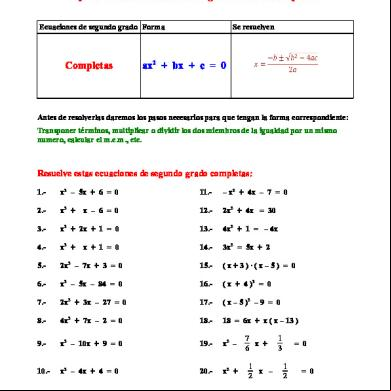
Ecuacion De Segundo Grado - Ejercicios 6d1t1o
January 2021 0
Imagenes Contenido Archivo Tratamientos Termicos Con Atmosfera Controlada Forjas Bolivar340 384a6h
November 2019 73
6l6m1j
April 2020 13
Shepsle Kenneth A. Y Mark S. Boncheck_analyzing Politics. Rationality, Behavior, And Institutions 6861g
December 2019 72